Numerical Optimization
An optimization problem is the problem of finding the best solution within a set of feasible solutions. There are many characteristics of optimization problems that define them and determine the methods needed to solve them. For example, we may have continuous or discrete problems; convex or non-convex problems; linear or non-linear problems. In this document we will consider continuous problems, and make no explicit assumptions on the convexity or the linearity of the problem. We will also focus on minimizing a function (maximizing \(f(x)\) is equivalent to minimizing \(-f(x)\)).
The general form of an optimization problem is \[\begin{alignat*}{3} & \text{minimize } \quad && f(x) \\ & \text{subject to } \quad && g_i(x) \leq 0, \quad && i = 1, \dots, m \\ & && h_j(x) = 0, \quad && j = 1, \dots, p, \end{alignat*}\] where \(f: \mathbb{R}^n \rightarrow \mathbb{R}\) is our objective function and \(g_i\) and \(h_j\) are our constraint functions.
The above formulation is a constrained optimization problem. We will consider unconstrained optimization in this document. Note that the R function optim offers L-BFGS-B for ‘box’ constrained optimization problems, and more options are supplied using constrOptim.
One-Dimensional Optimization
The optimization problem is rather difficult. Algorithms make it easy to find local optima, but finding global optima for non-convex problems is much harder. This is best illustrated by attempting to optimize a one-dimensional function. We can clearly see the global minimum in this scenario, but we cannot guarantee convergence to a global minimum with optimization algorithms.
Below we have plotted a simple curve which is periodic over \(2\pi\).
f <- function(x) {return(cos(x) + cos(2*x) + sin(2*x))}
curve(f, 0, 2*pi)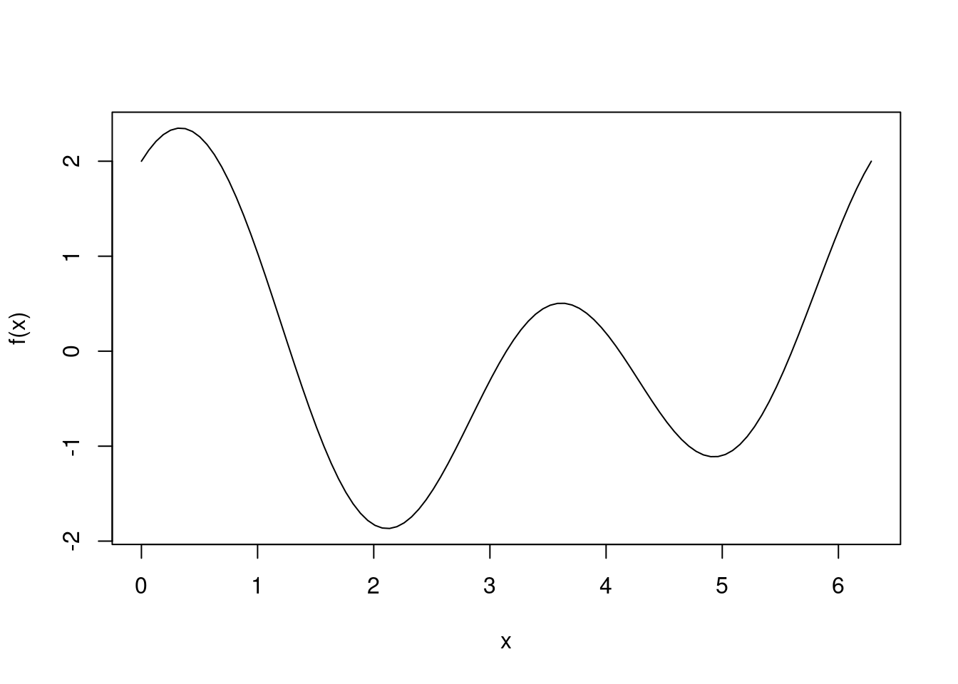
We can clearly see the global minimum is obtained at approximately 2, and a local minimum occurs around 5. We will test the optimize function in base R and see whether it finds the global minimum.
optimize(f, interval=c(0,2*pi))## $minimum
## [1] 2.116949
##
## $objective
## [1] -1.867534We see that optimize quickly found the global minimum in this case. However, if our interval is wider, optimize returns the local minimum.
optimize(f, interval=c(0,4*pi))## $minimum
## [1] 4.928807
##
## $objective
## [1] -1.112494The function optimize is based on golden section search, which works well for uni-modal functions. However, when a function has multiple extrema the golden section search method simply finds one of them and provides no assurance as to whether this is a global optimum point. It is useful in that it provides a derivative-free optimization method, which is incredibly fast and scales well.
In this case our function is one-dimensional meaning we can easily check whether we have indeed found the global minimum. However, when we have much higher-dimensional data it becomes nearly impossible to confirm whether we have found a global optimal point.
Newton’s method for optimization
Newton’s method aims to solve the unconstrained optimization problem:
\[\begin{alignat*}{3} & \text{minimize } \quad && f(x) . \end{alignat*}\]
In order to do this, we iteratively update \(x_k\), where \(x_{k+1}\) is chosen such that \[x_{k+1} = \text{argmin}_{x} f(x_k) + f'(x_k)(x - x_k) + \frac{1}{2}f''(x_k)(x - x_k)^2.\] Simply differentiating with respect to \(x\) and setting equal to zero, we see that \(x_{k+1} = x_k - \frac{f'(x_k)}{f''(x_k)}.\) Note that the update uses second-order information — the second derivative — and so converges faster. Newton’s method converges quadratically! It can also easily be rewritten for the multivariate case.
It’s important to note that at each iterate \(x_k\), Newton’s method chooses the next iterate \(x_{k+1}\) by minimizing a quadratic approximation of the true curve at \(x_k\).
We implement this in R and test the speed of convergence.
f_exp <- expression(cos(x) + cos(2*x) + sin(2*x))
f1_exp <- D(f_exp, 'x')
f1 <- function(x) eval(f1_exp)
f2_exp <- D(f1_exp, 'x')
f2 <- function(x) eval(f2_exp)
x <- 1.5
for(i in 1:5) {
  x <- x - f1(x)/f2(x)
  cat(x, '\n')
}
## 2.48044
## 1.987202
## 2.116103
## 2.116954
## 2.116954We see that our optimization algorithm converges in only three steps! Newton’s method is incredibly fast, and is only held back by the fact that we require the Hessian. It has computational complexity \(\mathcal{O}(n^3)\) as it needs to compute the inverse of the Hessian.
Here we demonstrate that at a given point, Newton’s method computes the quadratic approximation of the true curve at that point and minimizes it. We start close to the global minimum, with \(x_k = 1.7\). The quadratic approximation at \(x_k\) is plotted in blue, and we see that Newton’s method chooses \(x_{k+1}\approx2.2\).
cat("x_k = ", 1.7, "\n", sep="")## x_k = 1.7cat("x_k+1 = ", 1.7 - f1(1.7)/f2(1.7), sep="")## x_k+1 = 2.181084curve(f, 0, 2*pi)
second.order.approx <- function(x, xk) f(xk) + f1(xk)*(x-xk) + 1/2*f2(xk)*(x-xk)^2
seq <- seq(0,2*pi,length.out=100)
lines(seq, second.order.approx(seq, 1.7), col="blue")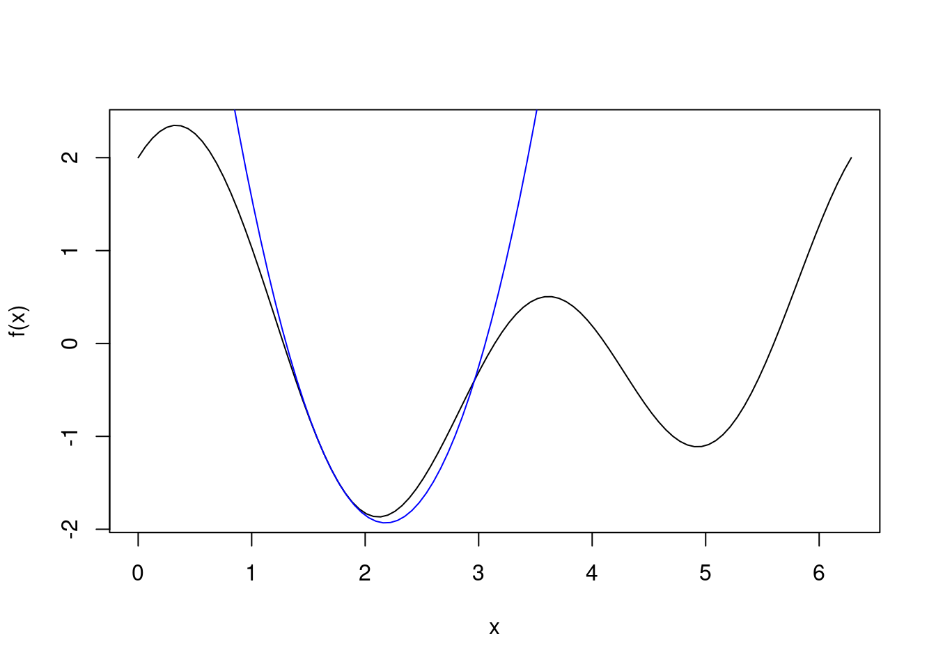
Newton’s method is also very dependent upon the starting point. We see below that if we were to initialize \(x\) at \(1\), then Newton’s method converges to the local minimum near \(x=5\). Under a different initialization at \(x=0.5\), the algorithm converges to the global maximum almost immediately. This occurs when our Hessian matrix becomes negative definite which corresponds to finding the maximum of a curve (recall that a sufficient condition for a strict local maximum (minimum) is that the Hessian is negative (positive) definite).
# initialized at 1
x <- 1
par(mfrow=c(1,4))
for(i in 1:4) {
  # compute updates
  x <- x - f1(x)/f2(x)
  cat("x", i, " = ", round(x, 2), "\n", sep="")

  # plot the approximation of the true curve at x1
  curve(f, -2*pi, 2*pi, ylim=c(-2,5), main="Quadratic approximation of f(x)")
  seq <- seq(-2*pi,2*pi,length.out=100)
  lines(seq, second.order.approx(seq, x), col="blue")
}
## x1 = -0.39## x2 = 2.96## x3 = 4.77## x4 = 4.94
# initialized at 0.5
x <- 0.5
par(mfrow=c(1,1))

# compute updates
x <- x - f1(x)/f2(x)
for(i in 1:3) {
  # compute updates
  x <- x - f1(x)/f2(x)
  cat("x", i, " = ", round(x, 2), "\n", sep="")
}
## x1 = 0.33
## x2 = 0.33
## x3 = 0.33# plot the approximation of the true curve at x1
curve(f, -2*pi, 2*pi, ylim=c(-2,5), main="Quadratic approximation of f(x)")
seq <- seq(-2*pi,2*pi,length.out=100)
lines(seq, second.order.approx(seq, x), col="blue")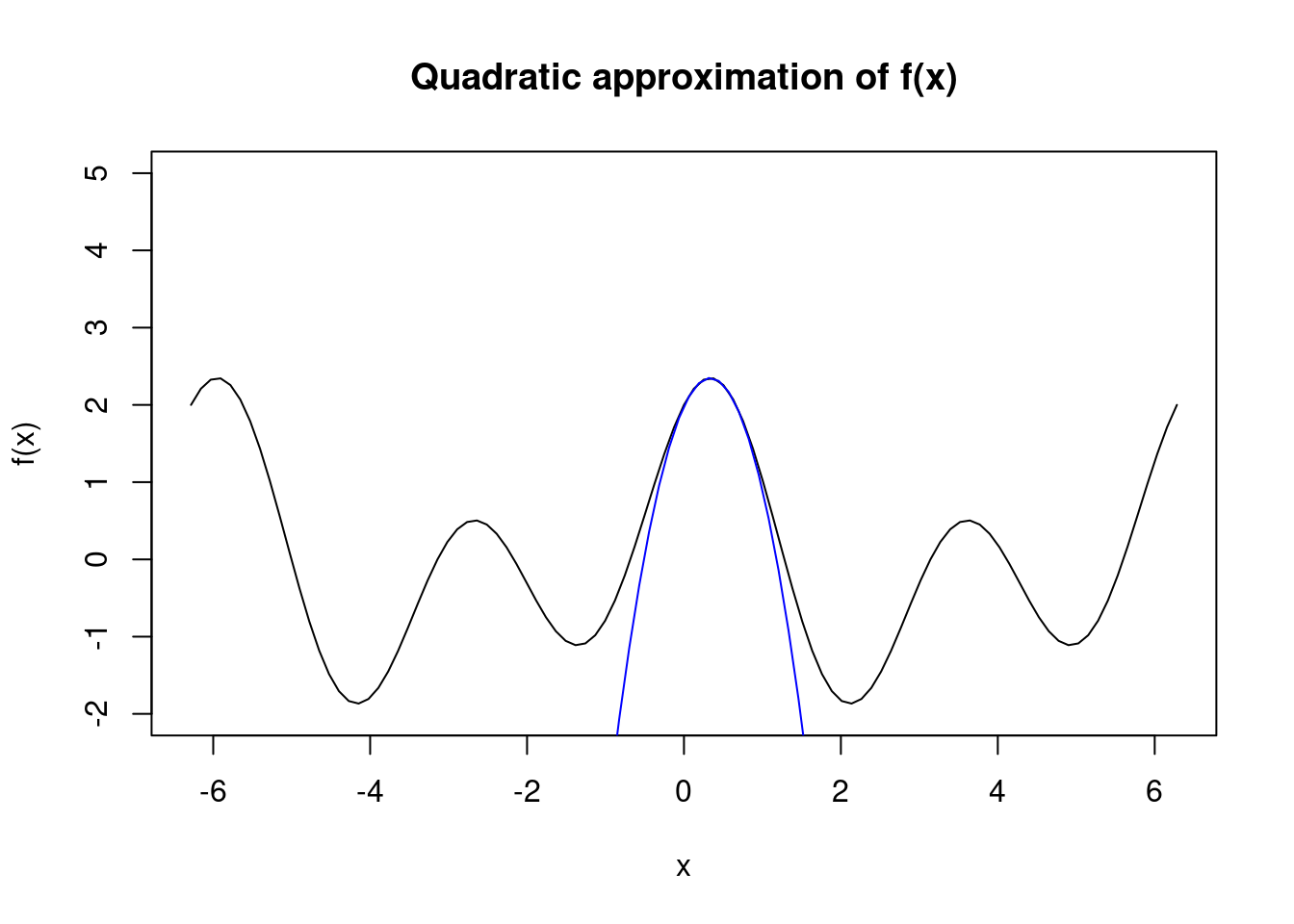
We have seen that one downside of Newton’s method is that it doesn’t differentiate between minima and maxima. It also requires the Hessian which can be difficult to produce for high-dimensional problems. The method presented above is known as pure Newton’s method, and there are variations which avoid these problems. To avoid finding local maxima we can ensure that the Hessian is positive (semi-) definite at each step, if it is not then we can modify it such that it is (e.g. we can add scalar multiple of the identity matrix to the Hessian such that it becomes positive definite, or we can take the eigendecomposition and modify the eigenvalues such that they are positive.). To avoid computing the Hessian we can use quasi-Newton methods which are similar to Newton’s method but they replace the exact Hessian with an approximation of the Hessian.
So far we have seen that one-dimensional unconstrained optimization is not as easy as we might expect. The problem becomes even more complex as the number of dimensions increase, and the computational complexity of our optimization algorithm becomes important.
Multi-dimensional optimization
Most of the objective functions we need to optimize are multi-dimensional. There are three common categories of optimization algorithms:
- Simplex methods — only uses the value of the function.
- First-order methods — uses the value of the function and the value of its first derivative. Gradient descent is a popular method within this category.
- Second-order methods — uses the value of the function, its first derivative, and its second derivative (the Hessian). Newton methods fall under this category.
The most popular method for multi-dimensional optimization in R is the optim function. optim implements a number of optimization algorithms such as Nelder-Mead, BFGS, CG (conjugate gradient), L-BFGS-B, SANN, and Brent. Another approach is to use the nlm (non-linear minimization) function, which uses a Newton-type algorithm.
Simplex methods
The Nelder-Mead algorithm is a well-known simplex method which is easily used in R.
Gradient-type methods
Gradient-type methods are much faster at converging than simplex methods, and avoid evaluating the Hessian. The most well-known method is steepest descent (gradient descent in the machine learning literature), in which we iteratively set \[x_{k+1} = x_k - \alpha \nabla f(x_k),\] where \(f(x)\), \(x \in \mathbb{R}^n\), is a differentiable and multivariate function, and \(\alpha\) is our step size (also known as learning rate). We can perform a line-search to find the optimal value of \(\alpha\) at each step. \(\alpha\) is often chosen to be a small value such as \(0.03\) but can be tuned to the specific problem. If our step size is too large the optimization algorithm will step beyond the optimal solution and could diverge.
Steepest descent converges slowly for high-dimensional problems but it has a very low computational cost. This is why steepest descent is the most widely-used optimization algorithm in the machine learning literature. When optimizing a neural network with hundreds of thousands of parameters, Newton’s method cannot be used due to its high computational cost (\(\mathcal{O}(n^3)\)). The computational cost of quasi-Newton methods is lower, but still cannot scale to such high-dimensional problems.
Gradient descent is well-known for its tendency to zigzag. Given its frequent use in machine learning, many improvements have been proposed in the machine learning literature. We will look at some of these proposals, implement them, and observe their rate of convergence.
We will consider the function \(f(x, y) = x^2 + 10y^2\). Below is a contour plot of this function.
# create contour plot
f <- function(x, y) {x^2 + 10*y^2}
s <- seq(-100,100,length=300)
contmat <- outer(s,
                 s,
                 Vectorize(function(x,y) f(x,y)))
rownames(contmat) <- colnames(contmat) <- s # keep x and y values and not the index
contlong <- melt(contmat) # melt into long format
## Warning in type.convert.default(X[[i]], ...): 'as.is' should be specified by the
## caller; using TRUE
## Warning in type.convert.default(X[[i]], ...): 'as.is' should be specified by the
## caller; using TRUEb <- exp(seq(log(10), log(100000), length = 25))
contplot <- contlong %>%
ggplot() +
geom_contour(aes(x = X1, y = X2, z = value, colour = stat(level)), breaks = b) +
ggtitle("Contour plot of f(x,y)") +
theme_minimal()
contplot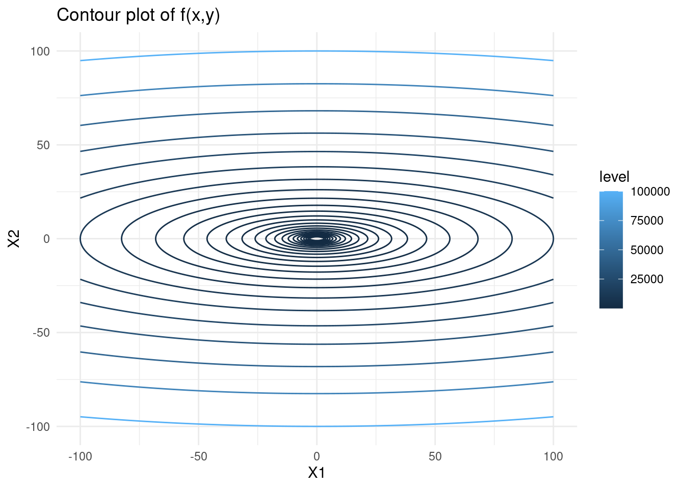
Let’s implement a simple version of steepest descent and view its zigzagging nature. We see that when the state space varies much more in one dimension than another, the algorithm tends to zigzag.
graddesc <- function(x0, fexp, iter, lr) {

  # get first derivative
  pars <- paste("x", 1:length(x0), sep="")
  f1 <- deriv(fexp, namevec = pars, function.arg = TRUE)

  # do gradient descent and keep all steps
  x_steps <- matrix(NA, iter+1, length(x0))
  x_steps[1,] <- x_gd <- x0
  for (i in 1:iter) {
    deriv <- attributes(do.call(f1, as.list(x_gd)))$gradient
    x_gd <- x_gd - lr * deriv
    x_steps[i+1,] <- c(x_gd)
  }

  return(x_steps)
}
f <- expression(x1^2 + 10*x2^2)
f_gd <- as.data.frame(graddesc(c(-100,-50), f, 20, 0.09))
contplot +
geom_line(data = f_gd, mapping = aes(x = V1, y = V2), colour = 'red') +
geom_point(data = f_gd, mapping = aes(x = V1, y = V2), shape = 21, colour = 'red') +
labs(subtitle = "using gradient descent")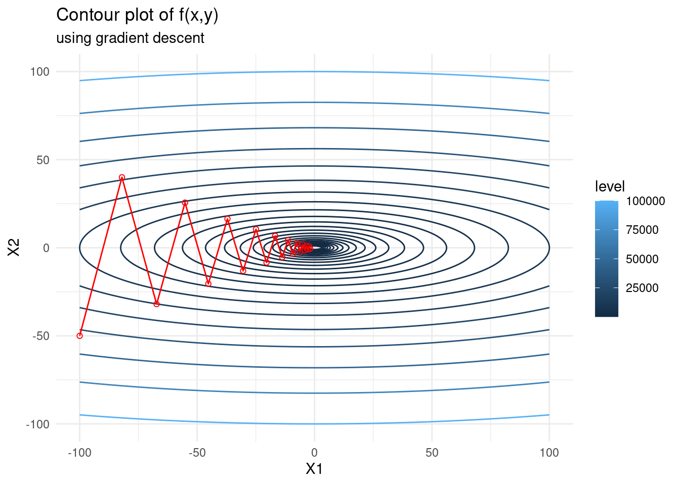
We see that for a non-optimal learning rate size (one that is too large) the gradient descent steps zigzag.
Gradient descent variants
Gradient descent with momentum
This method replaces the gradient of the objective function in the update with an exponentially weighted average of past gradients. This has the effect of smoothing out the update and dampens potential zigzagging. The iterative updates are \[\begin{alignat*}{2} x_{k+1} &= x_k - \alpha V_k \\ V_k &= \beta V_{k-1} + (1 - \beta)\nabla f(x_k), \end{alignat*}\] where \(\beta\) is a hyperparameter called the momentum, which ranges between 0 and 1. The larger the \(\beta\), the greater the smoothing effect. A popular choice for \(\beta\) is 0.9.
Momentum helps accelerate gradient descent by dampening oscillations. We will implement gradient descent with momentum and see if there is an improvement. Note that when \(\beta = 0\), gradient descent with momentum is simply gradient descent.
graddescmomentum <- function(x0, fexp, iter, lr, momentum) {

  # get first derivative
  pars <- paste("x", 1:length(x0), sep="")
  f1 <- deriv(fexp, namevec = pars, function.arg = TRUE)

  # do gradient descent and keep all steps
  x_steps <- matrix(NA, iter+1, length(x0))
  x_steps[1,] <- x_gd <- x0
  V <- rep(0,length(x0))
  for (i in 1:iter) {
    deriv <- attributes(do.call(f1, as.list(x_gd)))$gradient
    V <- momentum * V + (1 - momentum) * deriv
    x_gd <- x_gd - lr * V
    x_steps[i+1,] <- c(x_gd)
  }

  return(x_steps)
}

f <- expression(x1^2 + 10*x2^2)
f_gd <- as.data.frame(graddescmomentum(c(-100,-50), f, 20, 0.09, 0.5))
contplot +
  geom_line(data = f_gd, mapping = aes(x = V1, y = V2), colour = 'red') +
  geom_point(data = f_gd, mapping = aes(x = V1, y = V2), shape = 21, colour = 'red') +
  labs(subtitle = "using gradient descent with momentum")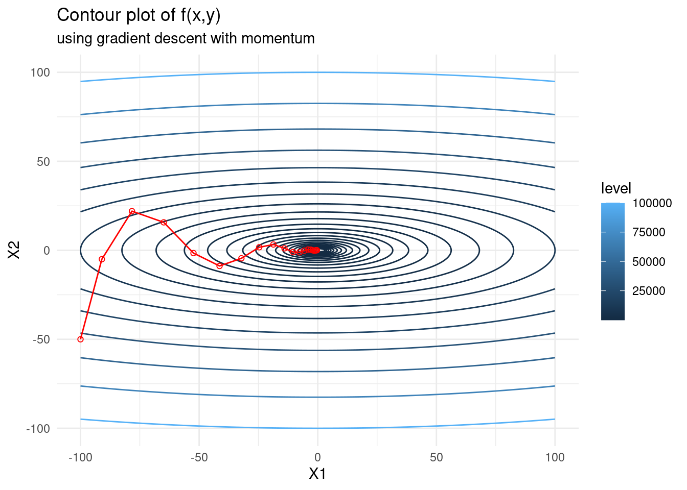
RMSprop
When finding the minimum point of a function, we may want to take large steps towards the minimum when we are far from it, and smaller steps when we are close. In order to achieve this we can employ a line search method, or a learning rate scheduler which decreases the learning rate at specified intervals. There are also methods which employ adaptive gradients, such as RMSprop.
The key idea of RMSprop is to store an exponentially weighted average of the squared gradients for each weight. RMSprop scales the gradient updates by dividing the learning rate by the square root of an exponentially decaying average of squared gradients — hence the name root mean-squared propagation.
RMSprop has the update formula \[\begin{alignat*}{2} x_{k+1} &= x_k - \frac{\alpha}{\sqrt{\nu_k + \epsilon}}\nabla f(x_{k}), \\ \nu_k &= \beta \nu_{k-1} + (1 - \beta) \nabla f(x_{k})^2, \end{alignat*}\] where \(\beta\) is the weighting of the moving average. A suggested default value for \(\beta\) is \(0.9\).
rmsprop <- function(x0, fexp, iter, lr, beta, eps = 1e-5) {

  # get first derivative
  pars <- paste("x", 1:length(x0), sep="")
  f1 <- deriv(fexp, namevec = pars, function.arg = TRUE)

  # do gradient descent and keep all steps
  x_steps <- matrix(NA, iter+1, length(x0))
  x_steps[1,] <- x_gd <- x0
  ms <- rep(0,length(x0))
  for (i in 1:iter) {
    deriv <- attributes(do.call(f1, as.list(x_gd)))$gradient
    ms <- beta * ms + (1 - beta) * deriv^2
    x_gd <- x_gd - (lr / sqrt(ms + eps)) * deriv
    x_steps[i+1,] <- c(x_gd)
  }

  return(x_steps)
}

f <- expression(x1^2 + 10*x2^2)
f_gd <- as.data.frame(rmsprop(c(-100,-50), f, 120, 1, 0.9))
contplot +
  geom_line(data = f_gd, mapping = aes(x = V1, y = V2), colour = 'red') +
  geom_point(data = f_gd, mapping = aes(x = V1, y = V2), shape = 21, colour = 'red') +
  labs(subtitle = "using RMSprop")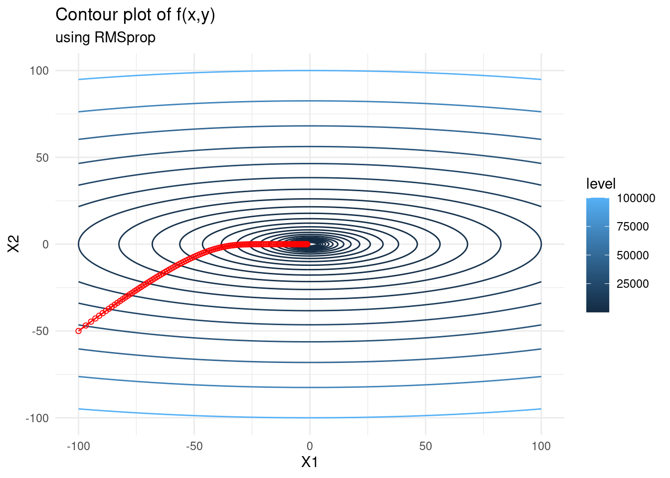
Adam
Adaptive Moment Estimation (Adam) also implements adaptive learning rates. Similar to RMSprop above, Adam stores an exponentially decaying average of squared gradients, and it also stores an exponentially decaying average of gradients similar to momentum.
Adams update formula is \[\begin{alignat*}{2} x_{k+1} &= x_k - \frac{\alpha}{\sqrt{\widehat{\nu}_k} + \epsilon}\widehat{m}_k, \\ m_k &= \beta_1 m_{k-1} + (1 - \beta_1) \nabla f(x_{k}),\\ \nu_k &= \beta_2 \nu_{k-1} + (1 - \beta_2) \nabla f(x_{k})^2,\\ \widehat{m}_k &= \frac{m_k}{1 - \beta_1^k},\\ \widehat{\nu}_k &= \frac{\nu_k}{1 - \beta_2^k}. \end{alignat*}\]
In the above, \(\beta_1\) and \(\beta_2\) are hyperparameters to be tuned. The original creaters of Adam propose default values of \(0.9\) for \(\beta_1\), \(0.999\) for \(\beta_2\), and \(10^{-8}\) for \(\epsilon\).
We can think of \(m_k\) and \(\nu_k\) as the first moment (the mean) and the second moment (the uncentered variance) respectively, hence the name adaptive moment estimation. As \(m\) and \(\nu\) are often initialized as (vectors of) zeros, they tend to be biased towards zero in the first few iterations. To avoid this bias towards zero we use \(\widehat{m}\) and \(\widehat{\nu}\) as specified above.
adam <- function(x0, fexp, iter, lr, beta1, beta2, eps = 1e-8) {

  # get first derivative
  pars <- paste("x", 1:length(x0), sep="")
  f1 <- deriv(fexp, namevec = pars, function.arg = TRUE)

  # do gradient descent and keep all steps
  x_steps <- matrix(NA, iter+1, length(x0))
  x_steps[1,] <- x_gd <- x0
  V <- S <- rep(0,length(x0))
  for (i in 1:iter) {
    deriv <- attributes(do.call(f1, as.list(x_gd)))$gradient
    V <- beta1 * V + (1-beta1) * deriv
    S <- beta2 * S + (1-beta2) * deriv^2
    Vhat <- V/(1-beta1^i)
    Shat <- S/(1-beta2^i)
    x_gd <- x_gd - lr / (sqrt(Shat) + eps) * Vhat
    x_steps[i+1,] <- c(x_gd)
  }

  return(x_steps)
}

f <- expression(x1^2 + 10*x2^2)
f_gd <- as.data.frame(adam(c(-100,-50), f, 100, 2, 0.9, 0.999))
contplot +
  geom_line(data = f_gd, mapping = aes(x = V1, y = V2), colour = 'red') +
  geom_point(data = f_gd, mapping = aes(x = V1, y = V2), shape = 21,
             colour = 'red', fill="white") +
  labs(subtitle = "using adam")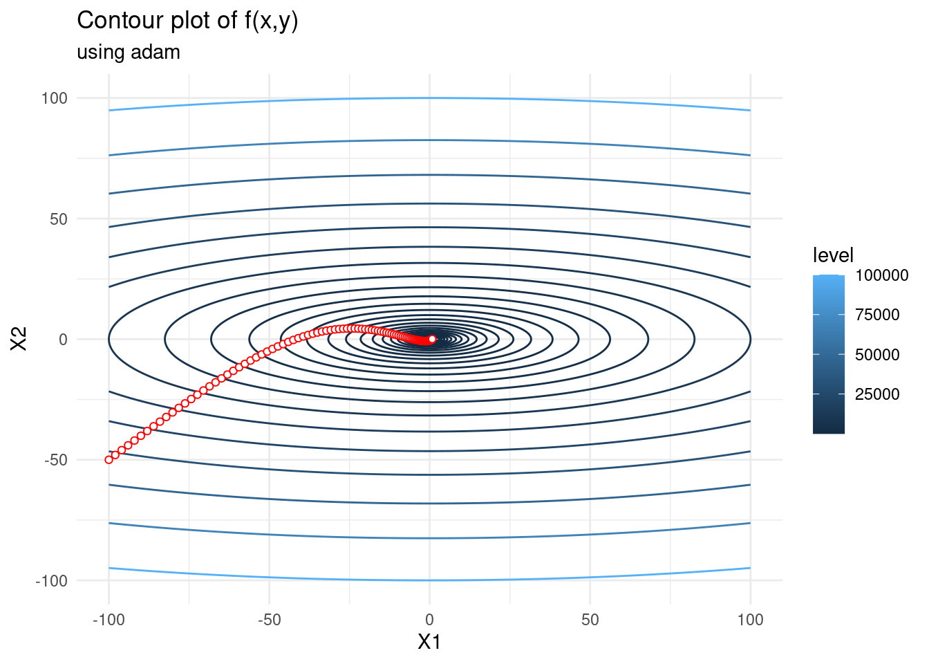
Second-order methods
Second-order methods converge much faster than first-order methods, but they also require more computation. We have already explained Newton’s method which is arguably the most widely-used second-order method, and so we will provide a brief summary here.
Newton’s method minimizes the quadratic approximation of \(f(x)\) around \(x_k\): \[Q(x) = f(x_k) + \nabla f(x_k)^T (x - x_k) + \frac{1}{2} (x - x_k)^T \nabla^2 f(x_k) (x - x_k)\] I.e. \(x_{k+1} = \text{argmin}_x Q(x)\). To find the minimum point we simply differentiate with respect to x and set equal to zero. This gives the update formula \[x_{k+1} = x_k - (\nabla^2 f(x_k))^{-1} \nabla f(x_k).\] We often include a step size parameter \(\alpha\) to control how large our steps are.
Newton’s method converges quadratically and has computational cost \(\mathcal{O}(n^3)\) for \(x \in \mathbb{R}^n\)
Pure Newton’s method may diverge if our initialization is bad. To avoid this we must ensure that our Hessian is positive (semi-) definite at each step, and ensure our step size is chosen such that the function decreases.
Computing the Hessian may be very difficult even if we use automatic differentiation. Storing the Hessian also becomes a problem for very high-dimensional problems.
Below we optimize \(f(x, y) = x^2 + 10y^2\) using Newton’s method. It converges in just \(1\) step! This is because the function is quadratic in two variables and thus the quadratic approximation to the true function computed by Newton’s method is exact. Newton’s method directly minimizes the true function in this case.
newton <- function(x0, fexp, iter, lr) {

  # get first and second derivative
  pars <- paste("x", 1:length(x0), sep="")
  d <- deriv(fexp, namevec = pars, function.arg = TRUE, hessian = TRUE)

  # do gradient descent and keep all steps
  x_steps <- matrix(NA, iter+1, length(x0))
  x_steps[1,] <- x_n <- x0
  ms <- rep(0,length(x0))
  for (i in 1:iter) {
    deriv <- attributes(do.call(d, as.list(x_n)))
    deriv_1 <- t(deriv$gradient)
    deriv_2 <- deriv$hessian[,,1:length(x0)]
    x_n <- x_n - lr*solve(deriv_2)%*%deriv_1
    x_steps[i+1,] <- c(x_n)
  }

  return(x_steps)
}

f <- expression(x1^2 + 10*x2^2)
f_n <- as.data.frame(newton(c(-100,-50), f, 5, 1))
contplot +
  geom_line(data = f_n, mapping = aes(x = V1, y = V2), colour = 'red') +
  geom_point(data = f_n, mapping = aes(x = V1, y = V2), shape = 21,
             colour = 'red', fill="white") +
  labs(subtitle = "using Newton's method")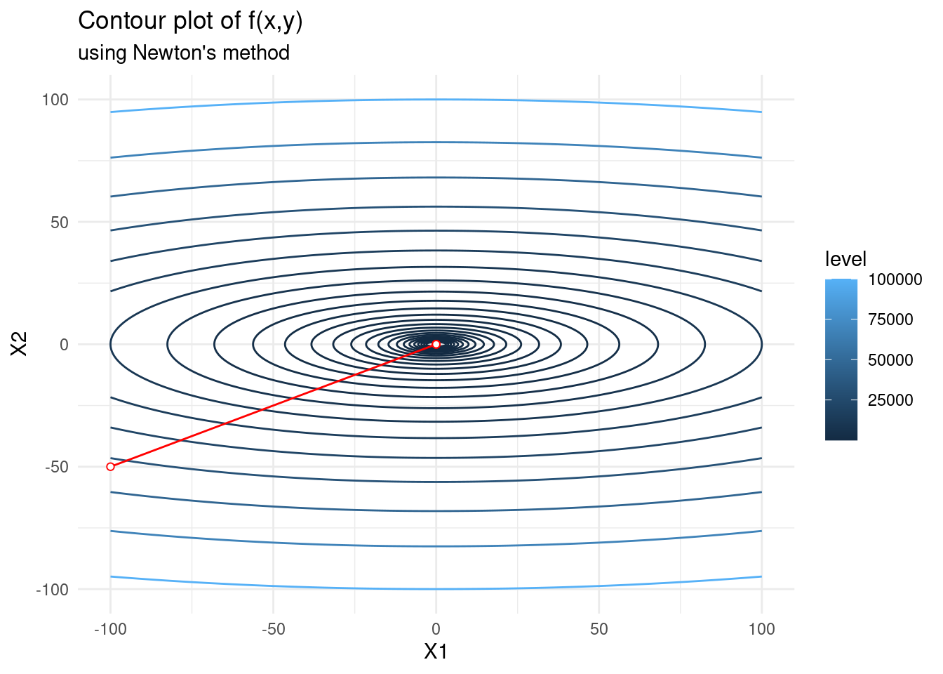
Quasi-Newton methods
Quasi-Newton methods are great substitutes for second-order methods. They approximate the Hessian at each iteration, rather than evaluate the true Hessian. This avoids the problem of computing the true Hessian for high-dimensional objective functions. Quasi-Newton methods are not as fast as Newton’s methods — they attain superlinear convergence. However, they also have a lower computational cost! They have complexity \(\mathcal{O}(n^2)\) whilst Newton’s method carries complexity \(\mathcal{O}(n^3)\).
BFGS is arguably the best quasi-Newton method which has been proposed thus far. It has update formula \(x_{k+1} = x_k - \alpha_k B_k \nabla f(x_k)\), where \(B_k\) is an \(n \times n\) symmetric positive definite matrix that is updated at each iteration and \(\alpha_k\) is our step size.
If we have a objective function with \(1000\) variables, the Hessian and its approximation is a \(1000 \times 1000\) dimension matrix. This is a large matrix to keep in memory and thus a limited-memory version of BFGS is often used (L-BFGS).
Let’s derive the BFGS update formula and see how it works. BFGS also works by minimizing the quadratic approximation of the true function around \(x_k\). Recall the Taylor series approximation of \(f(x_k + d)\) around \(x_k\). \[f(x_k + d) = f(x_k) + \nabla f(x_k)^T d + \frac{1}{2} d^T \nabla^2 f(x_k) d + o(\|d\|)^2\] We shall define the approximation of the objective function about \(x_k\) as \[m_k(d) := f(x_k) + \nabla f(x_k)^Td + \frac{1}{2}d^T B_k d,\] where \(B_k\) is an \(n \times n\) symmetric positive definite matrix which we will update. It is our approximation of the Hessian.
The minimizer of this convex quadratic \(m_k(d)\) is \(d = B_k^{-1} \nabla f(x_k)\). Hence we have the BFGS update formula \(x_{k+1} = x_k - \alpha_k B_k^{-1} \nabla f(x_k)\), where \(\alpha_k\) is our step size. The question now is: How do we compute \(B_k\)?
Instead of recomputing \(B_k\) at each iteration, we will update it based on information about the curvature gained in the most recent step. Suppose we observe a new iterate \(x_{k+1}\), then we form the quadratic approximation \(m_{k+1}(d) = f(x_{k+1}) + \nabla f(x_{k+1})^Td + \frac{1}{2}d^T B_{k+1} d\) In order to determine \(B_{k+1}\) we place restrictions on our approximation \(m_{k+1}(d)\). We want \(m_{k+1}(d)\) to be a good approximation to the objective function at \(x_{k+1}\). We propose that a good approximation will have the same gradient as the true function \(f\) at the two most recent iterates. That is, we require
\(\nabla m_{k+1}(0) = \nabla f(x_{k+1}),\)
\(\nabla m_{k+1}(- \alpha_k d_k) = \nabla f(x_{k+1}) - \alpha_k B_{k+1} d_k = \nabla f(x_k).\)
This first requirement is always true. The second requirement can be rewritten as \[\alpha_k B_{k+1} d_k = \nabla f(x_{k+1}) - \nabla f(x_{k}).\] Using the notation \(y_k = \nabla f(x_{k+1}) - \nabla f(x_{k})\), and \(s_k = x_{k+1} - x_k\) \((= \alpha_k d)\), we can rewrite the above equation as the secant equation \[B_{k+1}s_k = y_k.\] Note that if we approximate the Hessian we will then need to find its inverse to update \(x\). To avoid the expensive inversion, BFGS directly approximates the inverse of the Hessian which we will denote \(H\). Thus, we rewrite the secant equation \[ H_{k+1} y_k = s_k.\] This means that we require the symmetric positive definite matrix \(H_{k+1}\) to map \(y_k\) to \(s_k\). This is only possible if \(s_k\) and \(y_k\) satisfy the curvature condition: \(y_k^T s_k > 0\). If \(f\) is strongly convex then this is always true for any \(x_k\) and \(x_{k+1}\). If \(f\) is non-convex then we must impose this restriction explicitly. We can do this by imposing the (strong) Wolfe conditions on the line search for our step size.
The secant equations place \(n\) restrictions on \(H_{k+1}\), but we know that \(H_{k+1}\) is symmetric positive definite and thus has \(n(n+1)/2\) free parameters. Hence \(H_{k+1}\) has infinitely many solutions. In order to obtain a unique solution we must impose a further restriction. We require that among all symmetric matrices that satisfy the secant equation, \(H_{k+1}\) is in some sense closest to \(H_k\). We form the optimization problem \[\begin{alignat*}{2} &\text{minimize }_{H} \quad &&\| H - H_k \|, \\ &\text{subject to } && H = H^T, \\ & && H y_k = s_k, \end{alignat*}\] where \(s_k\) and \(y_k\) satisfy the curvature condition and \(H_k\) is symmetric and positive definite.
Different matrix norms result in different quasi-Newton methods. A norm which provides an easy solution to the optimization problem which is also scale-invariant is the weighted Frobenius norm \[\|A\|_W = \|W^{1/2}AW^{1/2}\|_F,\] where \(\|\cdot\|_F\) is defined by \(\|A\|_F = \sum_{i=1}^n\sum_{j=1}^n a_{ij}^2\).
The matrix W can be chosen to be any matrix satisfying \(Ws_k = y_k\). One possible \(W\) which we know gives a solution is the inverse of the average Hessian. That is, \[W = \bar{G}_k^{-1}, \quad \text{where } \bar{G}_k = \int_0^1 \nabla^2 f(x_k + t \alpha_k d_k) dt.\]
The choices above: the weighted Frobenius norm and \(W\) the inverse of the average Hessian provide the following unique solution to the optimization problem
\[H_{k+1} = (I - \rho_k s_k y_k^T) H_k (I - \rho y_k s_k^T) + \rho_k s_k s_k^T,\] where \(\rho_k = \frac{1}{y_k^T s_k}\).
Given this update formula for \(H_{k+1}\), the resulting BFGS algorithm is quite simple!
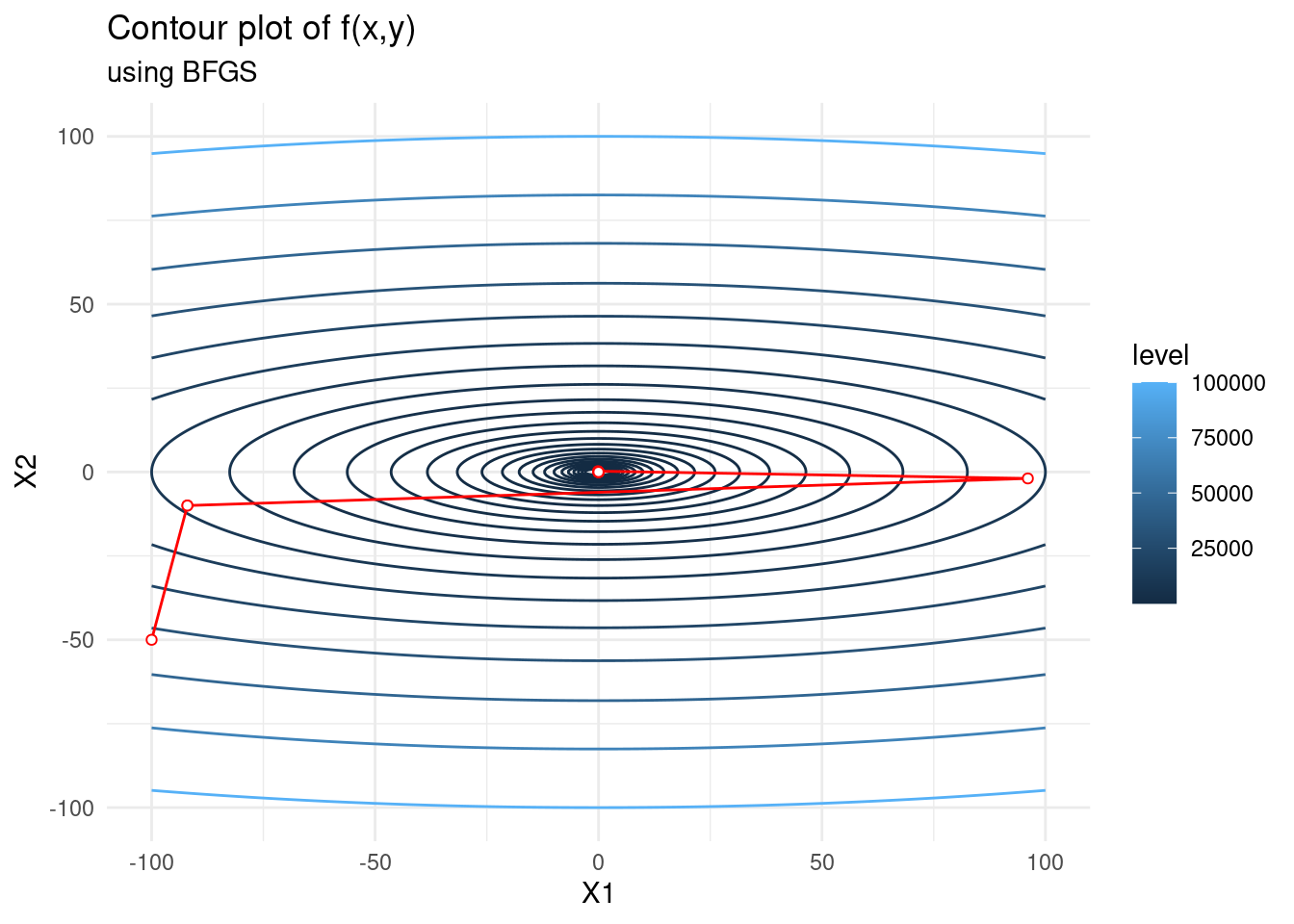
Below we continue to optimize the function \(f(x, y) = x^2 + 10y^2\). We use BFGS and see that it converges in only 3 steps! Clearly it is far superior to first-order methods when the objective function has a reasonable number of parameters. This is of course not an easy number to quantify, but well-defined objective functions with a large number of parameters can be optimized with BFGS.
f <- function(x) {(x[1]^2 + 10*x[2]^2)}
f_bfgs <- c(-100,-50)
for(i in 1:10) {
  f_bfgs <- rbind(f_bfgs, optim(c(-100,-50), f,
                                method = "BFGS", control=list(maxit=i))$par)
}
f_bfgs <- as.data.frame(f_bfgs, row.names=1:11)
contplot +
  geom_path(data = f_bfgs, mapping = aes(x = V1, y = V2), colour = 'red') +
  geom_point(data = f_bfgs, mapping = aes(x = V1, y = V2), shape = 21,
             colour = 'red', fill="white") +
  labs(subtitle = "using BFGS")