Example of debugging

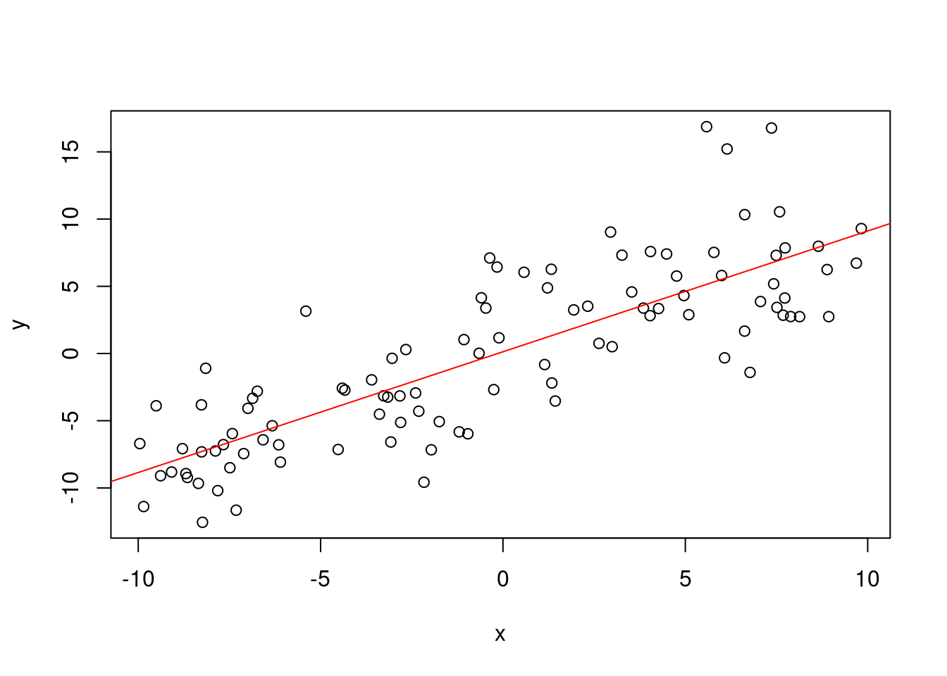
Consider an example in which we have a dataset of pairs of observations \(\{x_i, y_i\}_{i=1}^n\). We will generate this data using \(x_i \sim U[-10,10],\) for \(i=1,\dots,n\), and \(y_i = x_i + \epsilon_i\), where \(\epsilon \sim N(0,4)\). We will fit a linear model with the covariate \(x\). We will clumsily implement the least squares solution.

x <- runif(100,-10,10)
y <- (x) + rnorm(100,0,4)

# built-in function
model <- lm(y~x)
plot(x,y)
abline(model$coefficients, col="red")

linear_regression <- function(X,y) {
  beta <- solve(X %*% t(X)) %*% t(X) %*% y
  return(beta %*% X)
}
x <- cbind(rep(1,100), x)
linear_regression(x, y)

## Error in solve.default(X %*% t(X)): system is computationally singular: reciprocal condition number = 1.95111e-22

We cannot perform the matrix inverse as our system is computationally singular. There are a number of reasons that this may have happened, but I suspect that there may simply be a transpose where there shouldn’t be. However, there may also be a larger problem. In some cases our variables within the function are not what we expect them to be. In this case we are trying to compute \((XX^T)^{-1}\), when we should be computing \((X^TX)^{-1}\).

We can use the traceback() function to find out what caused the error. We see that the error stems from the solve.default() function.

traceback()

## No traceback available

The RStudio IDE provides great resources for debugging. An intuitive method one may implement is to place multiple print(<variable>)s in the function to determine the value of different variables. A much more effective method is to place broswer() within your code. This opens an interactive debugging environment.

My preferred method of debugging code is to enter debug(<function>) into the console. Then when the specified function is ran we will immediately enter the interactive debugging environment within RStudio. When coding non-trivial functions this is life changing. This is always my first suggestion when someone can’t find a bug in their code. You can go through the function’s computation line-by-line, and print variables’ values via the console.

It clearly isn’t possible to demonstrate the interactive environment within this document. However if we were in the interactive environment, we would see that solve(t(x) %*% x) is possible.

linear_regression <- function(X,y) {
  beta <- solve(t(X) %*% X) %*% t(X) %*% y
  return(beta %*% X)
}
linear_regression(x, y)

## Error in beta %*% X: non-conformable arguments

We have solved one problem, but we have another. We now have non-conformable arguments. If we enter the interactive debugging environment we can see that beta has dimension (2,1) and X has dimension (100,2). Clearly this matrix multiplication isn’t possible — we should be computing X %*% beta. This produces a column vector of predictions.

linear_regression <- function(X,y) {
  beta <- solve(t(X) %*% X) %*% t(X) %*% y
  return(X %*% beta)
}
linear_regression(x, y)[1:5]

## [1] -6.893672 -6.754188 -6.950980  6.880512 -6.034347

We have successfully output predictions!

Example

Here we will use kernel regression as an example. We quickly recall the kernel method setup:

Our estimator takes the form \[ f(x; w_{LS-R}) = k(K + \lambda I)^{-1}y^T \] where \(k^{(i)} = k(x, x_i) = \langle \phi(x), \phi(x_i)\rangle\), \(K_{i,j} = k(x_i, x_j)\).

We have many choices for the kernel function \(k\):

• Linear kernel function: \(k(x_i, x_j) = \langle x_i, x_j \rangle\),

• Polynomial kernel function (of order \(b\)): \(k(x_i, x_j) = (\langle x_i, x_j \rangle + 1)^b\),

• Radial basis function kernel: \(k(x_i, x_j) = \frac{\|x_i - x_j\|^2}{\sigma^2}\).

We will implement a kernel method using the radial basis function. In this first implementation we are going to compute the \(n \times n\) matrix \(K\) by using two for loops. This function will produce one prediction at a time, and so we must loop over it a number of times in order to make more than one prediction. Note: We must recompute our estimator for every prediction.

rbf_function <- function(vec1, vec2, bandwidth) {
  return(exp(-norm(vec1 - vec2, type = "2")^2/bandwidth^2))
}

kernel_regression_1 <- function(X, y, x.pred, lambda, bandwidth) {
  n <- ncol(y)
  n.pred <- ncol(x.pred)
  k <- c()
  for (i in 1:n) {
      k <- c(k, rbf_function(x.pred, X[,i], bandwidth))
  }

  K <- matrix(nrow=n, ncol=n)
  for (i in 1:n) {
    for (j in 1:n) {
      K[i,j] <- rbf_function(X[,i], X[,j], bandwidth)
    }
  }
  return(k %*% solve(K + lambda * diag(1,n)) %*% t(y))
}

We simulate some basic data in order to evaluate the function.

set.seed(123)
X <- matrix(runif(100), ncol=100)
X <- rbind(X, rep(1,100))
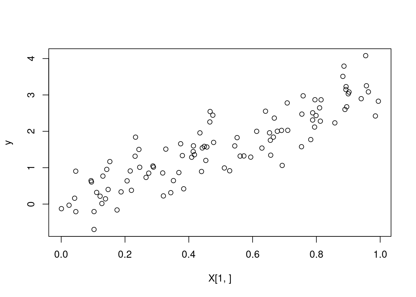
y <- matrix(3.2*X[1,] + rnorm(100,0,0.5), ncol=100)

# a wrapper function which allows us to produce multiple predictions
multiple_pred <- function(X, y, x.pred, lambda, bandwidth) {
  pred <- c()
  for (i in 1:ncol(x.pred)) {
    pred <- c(pred, kernel_regression_1(X, y, x.pred[,i], lambda, bandwidth))
  }
  return(pred)
}

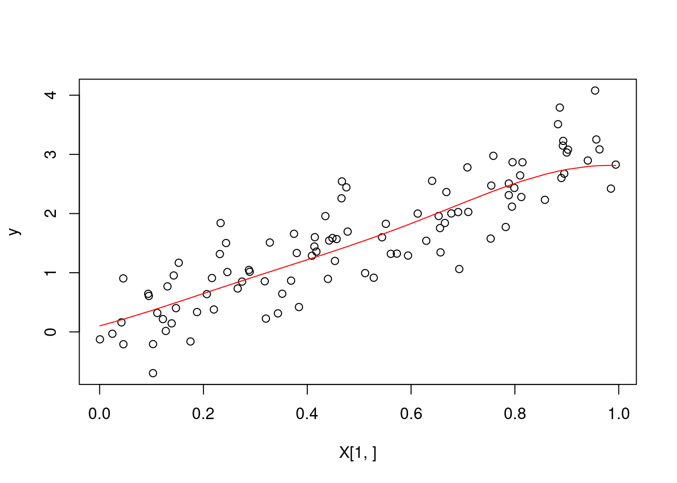
# sanity check --- we plot our predicted values
predictions <- multiple_pred(X, y, X, 1, 0.5)
plot(X[1,], y)
lines(sort(X[1,]), predictions[order(X[1,])], col = "red")

# we use profvis to analyse the code
profvis(multiple_pred(X, y, X, 1, 0.5))

We see that the function kernel_regression_1 is extremely inefficient. The biggest problem occurs due to the number of calls to the rbf_function. We will rewrite the function such that we only compute the \(n \times n\) matrix once (for any number of predictions), and rerun the profvis analysis.

kernel_regression_2 <- function(X, y, x.pred, lambda, bandwidth) {
  n <- ncol(y)
  n.pred <- ncol(x.pred)
  k <- matrix(nrow=n.pred, ncol = n)
  for (i in 1:n.pred) {
    for (j in 1:n) {
      k[i,j] <- rbf_function(x.pred[,i], X[,j], bandwidth)
    }
  }

  K <- matrix(nrow=n, ncol=n)
  for (i in 1:n) {
    for (j in 1:n) {
      K[i,j] <- rbf_function(X[,i], X[,j], bandwidth)
    }
  }
  return(k %*% solve(K + lambda * diag(1,n)) %*% t(y))
}

# sanity check --- we plot our predicted values
predictions <- kernel_regression_2(X, y, X, 1, 0.5)
plot(X[1,], y)
lines(sort(X[1,]), predictions[order(X[1,])], col = "red")

# profvis
profvis(kernel_regression_2(X, y, X, 1, 0.5))

We see a speedup of approximately 45 times! The memory is also much more optimized. The majority of our computation time is still determined by the calls to the rbf_function. We see it is being used in two sets of nested for loops. Perhaps we could avoid this by vectorization. We will attempt to instead compute the outer product of arrays.

kernel_regression_3 <- function(X, y, x.pred, lambda, bandwidth) {
  n <- ncol(y)
  n.pred <- ncol(x.pred)
  k <- matrix(nrow=n.pred, ncol = n)

  K <- outer(
    1:n, 1:n,
    Vectorize(function(i,j) rbf_function(X[,i], X[,j], bandwidth))
  )

  return(k %*% solve(K + lambda * diag(1,n)) %*% t(y))
}

# sanity check --- we plot our predicted values
predictions <- kernel_regression_3(X, y, X, 1, 0.5)
plot(X[1,], y)
lines(sort(X[1,]), predictions[order(X[1,])], col = "red")

# profvis
profvis(kernel_regression_3(X, y, X, 1, 0.5))

Memory management in R

R uses pass-by-value semantics in its function calls. This means that if we assign some variable \(x\) to be equal to another variable \(y\), then changing the value of \(y\) will not change the value of \(x\). Code in R is interpreted line-by-line. This means that coding in R is rather intuitive and easy to reason about, but it also means that the code produced may not perform well — particularly in comparison to languages such as C which implement pass-by-reference semantics. After algorithmic complexity, memory management is one of the most important factors in performance.

There are many things that R does in the background to improve performance. When editing elements in a matrix it seems illogical to work with multiple copies of the matrix, and so R indexes into the element and modifies it in place. In some cases R will copy the matrix and modify it.

library(pryr)

# modify in place
x <- rep(1,2)
x[2] <- 2

# assign y to be x
y <- x

# show y is not a copy of x --- R just points to x
# refs(x) tells us how many variables point to this location
c(address(x), refs(x))

## [1] "0x55e2a1289448" "3"

When refs() is 1 then R will modify the array in place. When refs() is 2 or greater, R will copy the array and modify the copy. This will prevent modifying an array that other variables are pointing to. This can be seen below.

x <- rep(1,10)
c(address(x), refs(x))

## [1] "0x55e2a13be8d8" "2"

z <- x
c(address(x), refs(x))

## [1] "0x55e2a13be8d8" "4"

x[5] <- 2
c(address(x), refs(x)) # creates a copy of x and modifies it

## [1] "0x55e2a13bf958" "1"

When writing code it is best to avoid creating copies of an array as this is an inefficient use of memory. If you are worried about memory efficiency you should routinely use address() and refs() in order to test when objects are being copied. It may be useful to know that primitive functions in R do not increment the refs() count, whereas all non-primitive functions increment the refs() count. If memory efficiency is very important to you, it may be better to use Rcpp and write your function in C++.

# modifies in place because <- <vector> is a primitive function
x <- 1:5
for(i in 1:5) {
  x[i] <- x[i] - 1
  print(c(address(x), refs(x)))
}

## [1] "0x55e2a1a2e248" "1"             
## [1] "0x55e2a1a2e248" "1"             
## [1] "0x55e2a1a2e248" "1"             
## [1] "0x55e2a1a2e248" "1"             
## [1] "0x55e2a1a2e248" "1"

# creates a copy because <- <data.frame> is not a primitive function
# we must be careful when working with non-primitive data structures
# problem occurs because refs counter is incremented and thus R
# copies the object
x <- data.frame(1:5)
for(i in 1:5) {
  x[i,1] <- x[i,1] - 1
  print(c(address(x), refs(x)))
}

## [1] "0x55e2a18eed50" "1"             
## [1] "0x55e2a18f01e0" "1"             
## [1] "0x55e2a1453008" "1"             
## [1] "0x55e2a1446a58" "1"             
## [1] "0x55e2a1447e08" "1"