Programming paradigms
R supports multiple programming paradigms. Programming paradigms describe the way in which code is written and structured for larger projects. The types of programming structures are:
- Imperative programming — We define a sequence of instructions that modify the ‘state’ of the program.
- Object-oriented programming — Objects combine the machine’s state with a set of methods. Programs are then defined via the construction of objects.
- Declarative programming — A sequence of operations is defined that only specify what the output of the program should be. The exact details of how the program is implemented is determined by the programming language.
- Functional programming — Functions are defined to act identically to mathematical functions. A program is then a sequence of function applications.
In this document we will explore the use and applications of functional and object-oriented programming.
Functional programming
First-class functions
R has first-class functions. These are functions that behave like any other data structure. A language has first-class functions if:
- Functions can be used as arguments to other functions,
- Functions can be returned by functions,
- Functions can be stored in data structures.
In functional programming we may want to provide a function as an input to another function. We have seen this feature in the Map and Reduce functions in R.
square <- function(x) x*x
unlist(Map(square, 1:5))
## [1] 1 4 9 16 25Reduce('+', 1:5)## [1] 15Reduce('+', unlist(Map(square, 1:5)))## [1] 55# we can also use multiple functions within one function
Reduce(function(x,y) x*y, unlist(Map(square, 1:5)))## [1] 14400We can also take a function as an input, manipulate it, and return it as an output.
Object-oriented programming
Introduction
The main reason to use object-oriented programming (OOP) is polymorphism. This provides our functions with reusability and extendability. Polymorphism allows a single object to have multiple methods for various types of input.
In OOP, functionality is encapsulated within an object. Every object has a type, which is the class that it belongs to. An implementation for a specific class is called a method. The class defines the fields, which contain the data possessed by every instance of that class. The current state of an object is thus specified by its fields, and its behavior is specified by its methods. If one class is derived from the other, the child class may inherit the fields and methods of the parent class.
R implements three different object-oriented systems:
- S3 — An informal implementation of OOP which relies upon common conventions.
- S4 — A formal rewrite of S3.
- Reference classes (RC) — Implements encapsulated OOP. In this implementation objects are mutable. That is, objects are modified in place.
In this report we will look at the S3 and S4 systems.
S3
S3 is the simplest and most informal system for OOP in R. S3 does not use formal class definitions. It offers an extremely flexible system, which may allow you to do certain things which are not recommended. Since S3 has few built-in constraints, we will outline best practices here.
An S3 object is an object of a base type with the attribute class set to the class name. It will be good practice to have a constructor function which can be called to initialize all relevant elements of the object, and then return the object. We may also require a validator which checks our arguments within a separate function. A helper function is also useful for end users that makes the constructor more user-friendly.
Below we will implement linear regression as an S3 object.
# we set the seed for reproducibility
set.seed(1)

# create a dataset
n <- 100
w <- matrix(c(2, -1), ncol=1)
X <- rbind(rnorm(100,0,1), rep(1,n))
y <- t(w)%*%X + rnorm(100, 0, 1)
plot(X[1,], y[1,])
# we now define a constructor which will return an object of a specified class
# the constructor does some operations
# encapsulates data in the object
# assigns a class to the object
# returns the object
simple_lin_regression <- function(X, y) {

  # compute the OLS parameter estimates
  w_hat <- solve(X%*%t(X))%*%X%*%t(y)

  # the object encapsulates (X, y, and w_hat)
  slr <- list(response = as.numeric(y), regressor = X, param_estimate = w_hat)

  # we declare the object 'slr' to be an S3 object of class "simple_lin_regression"
  class(slr) <- "simple_lin_regression"

  return(slr)
}

slr <- simple_lin_regression(X, y)
Given the above class simple_lin_regression, we will define some methods for the class. To define a method in S3, a generic function of the same name needs to already exist. If it doesn’t already exist we can easily declare a new generic function.
We define a new method as a function with function name [method_name].[class_name].
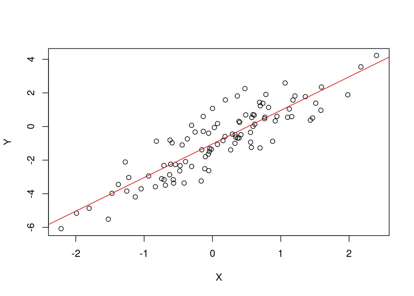
We implement a print method which prints relevant information about the object such as the estimated coefficients, and we implement a plot method. Note that print and plot are already generic methods in R and so we do not need to define them as such here.
print.simple_lin_regression <- function(x, ...) {
  cat("head(x) =", head(x$regressor[1,]), "\n")
  cat("head(y) =", head(x$response), "\n")
  cat("Estimated regression: E[y|x] = b0 + b1*x\n")
  cat("b0 = ", x$param_estimate[1,1], ", b1 = ", x$param_estimate[2,1], ".\n", sep="")
}

plot.simple_lin_regression <- function(x, ...) {
  plot(x$regressor[1,], slr$response,
       xlab=expression(X), ylab=expression(Y)
  )
  abline(a = x$param_estimate[2], b = x$param_estimate[1], col = "red")
}
Let’s use the methods we defined above. The correct syntax is [method_name](object]).
print(slr)## head(x) = -0.6264538 0.1836433 -0.8356286 1.595281 0.3295078 -0.8204684
## head(y) = -2.873274 -0.5905975 -3.582179 2.34859 -0.9955691 -0.8736495
## Estimated regression: E[y|x] = b0 + b1*x
## b0 = 1.99894, b1 = -1.037693.plot(slr)
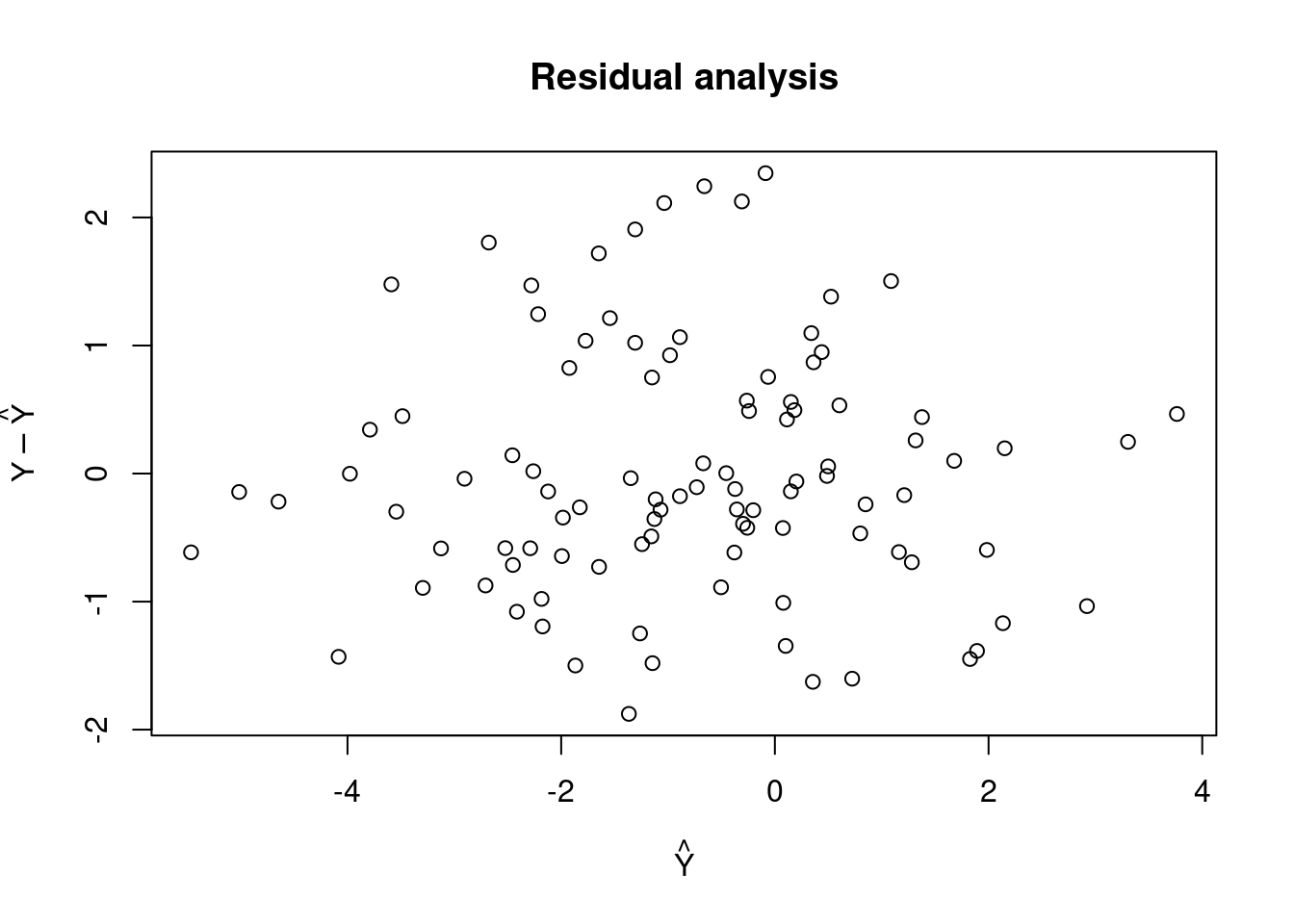
We want to define a method called residual_analysis. In order to do this we must define a generic method with the same name.
# define the generic method
residual_analysis <- function(x){
  UseMethod("residual_analysis")
}

# implement the method for class
residual_analysis.simple_lin_regression <- function(x) {
  predictions <- t(x$param_estimate) %*% X
  plot(predictions, x$response - predictions,
       main = "Residual analysis",
       xlab = expression(hat(Y)), ylab = expression(Y-hat(Y)))
}

residual_analysis(slr)
In S3, classes can inherit methods from their parent classes. This is demonstrated below. Note that we can create classes on the fly — we not need to formally define them. We simply define an object and then assign its class.
P <- structure(numeric(), class = "parent_class")
C <- structure(numeric(), class = c("child_class", "parent_class"))

print.parent_class <- function(x) {
  cat("This method belongs to the parent class")
}
We check that the method works for both P and C.
print(P)## This method belongs to the parent classprint(C)## This method belongs to the parent classWe now provide the child_class class with its own print method.
print.child_class <- function(x) {
  cat("This method belongs to the child class")
}

print(C)
## This method belongs to the child classprint(P)## This method belongs to the parent classprint(C)## This method belongs to the child classS4
S4 implements a more formal approach to OOP. Unlike S3, all OOP relevant elements must be defined explicitly. S4 provides specialized functions for defining elements such as setClass(), setGeneric(), and setMethod(). While this requires more effort, it provides more clarity and allows us to use built-in integrity checks.
We repeat the linear regression task.
library(methods)We must first create the simple_lin_regression class. We must give it the name of the class being defined, and the slots which represent the fields’ names and types. Slots can be accessed using the specialized subsetting operator @, however we should avoid using this outside of methods in order to provide encapsulation. In order to obtain or change an object’s components we should use getter and setter methods which we define.
setClass("simple_lin_regression",
         slots = c(
           response = "numeric",
           regressor = "numeric",
           estimate = "numeric"
         )
)
We can instantiate a new object in the class using new(). We create a constructor so that the end user does not have to use the new function.
simple_lin_regression <- function(X,y) {
  slr <- new("simple_lin_regression",
             response = y,
             regressor = X)
  return(slr)
}
We quickly test that our constructor function works for our generated data.
slr <- simple_lin_regression(X[1,1:5],y[1,1:5])
slr
## An object of class "simple_lin_regression"
## Slot "response":
## [1] -2.8732743 -0.5905975 -3.5821789 2.3485904 -0.9955691
##
## Slot "regressor":
## [1] -0.6264538 0.1836433 -0.8356286 1.5952808 0.3295078
##
## Slot "estimate":
## numeric(0)Note that the slot for estimate exists but we have not given it a value yet. It is currently numeric(0). We will create an initialization method that will compute the estimate when we create an object.
setMethod("initialize", "simple_lin_regression",
          function(.Object, response, regressor) {
            .Object@response <- response
            .Object@regressor <-  regressor

            n <- length(response)
            X <- rbind(regressor, rep(1,n))
            w_hat <- solve(X%*%t(X))%*%X %*% response
            .Object@estimate <- as.numeric(w_hat)
            return(.Object)
          })
When we use the function new() we see that it calls a non-standard generic function initialize(). We can define a custom initialize method that assigns values (such as default values) to an object’s components. We can also perform a computation like above and set its output to one of the object’s components. The first two arguments in the above specify the method initialize, and the class for which it is defined for simple_lin_regression. It returns the object .Object with the components it has been assigned.
Similar to what we did for S3, we implement print and pot functions for S4. Recall that in order to access the components of our object we must use the @ operator.
setMethod("print", "simple_lin_regression",
  function(x, ...) {
    cat("head(x) =", head(x@regressor), "\n")
    cat("head(y) =", head(x@response), "\n\n")
    cat("Estimated regression: E[y|x] = b0 + b1 * x\n")
    cat("b0 = ", x@estimate[1], " and b1 = ", x@estimate[2], ".\n", sep = "")
  }
)

setMethod("plot", "simple_lin_regression",
  function(x, y = NULL, ...) {
    plot(x = x@regressor, y = x@response,
         xlab = expression(X), ylab = expression(Y))
    abline(a = x@estimate[2], b = x@estimate[1], col = "red")
  }
)
slr <- simple_lin_regression(X[1,], y[1,])
print(slr)## head(x) = -0.6264538 0.1836433 -0.8356286 1.595281 0.3295078 -0.8204684
## head(y) = -2.873274 -0.5905975 -3.582179 2.34859 -0.9955691 -0.8736495
##
## Estimated regression: E[y|x] = b0 + b1 * x
## b0 = 1.99894 and b1 = -1.037693.plot(slr)
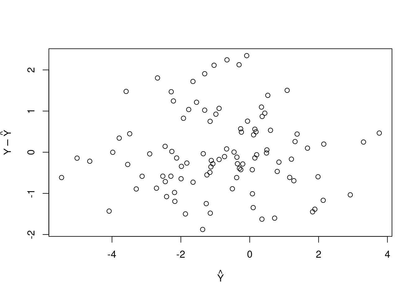
Once again, we implement a method called residual_analysis which is a not a generic method and must be defined using setGeneric().
setGeneric("residual_analysis")## [1] "residual_analysis"setMethod("residual_analysis", "simple_lin_regression",
function(x) {
predictions <- x@estimate[2] + x@estimate[1] * x@regressor
plot(x = predictions, y = x@response - predictions,
xlab = expression(hat(Y)),
ylab = expression(Y - hat(Y)))
})
residual_analysis(slr)
Monte carlo example of S4
We will implement Monte Carlo integration using S4.
We start with the general problem: We want to compute an integral \[ \mathbb{E}_f[h(X)] = \int_\mathcal{X} h(x) f(x) dx \] where \(\mathcal{X}\) is the set from which the random variable \(X\) takes its values. In order to compute this integral numerically, we are going to generate a sample \((X_1, \dots, X_n)\) from the density \(f\) and approximate the integral via the empirical mean \[ \bar{h}_n := \frac{1}{n} \sum_{i=1}^n h(x_i).\] This is a logical estimator as \(\bar{h}_n \rightarrow \mathbb{E}_f[h(X)]\) as \(n \rightarrow \infty\) almost surely (by the Strong Law of Large Numbers).
We implement the above method in a class called monteCarloIntegration.
setClass("monteCarloIntegration",
         slots = c(
           func = "function",
           lower_lim = "numeric",
           upper_lim = "numeric",
           estimates = "numeric",
           est_errors = "numeric"
         ))
We now create a constructor function.
monte_carlo_int <- function(func, lower, upper) {
  monte_carlo_integral <- new("monteCarloIntegration",
                              func = func,
                              lower_lim = lower,
                              upper_lim = upper)
  return(monte_carlo_integral)
}
Let’s test that our constructor works. We are going to integrate the function \[h(x) := [\cos(10x) + sin(4x)]^3\] over [0,1].
h <- function(x) {(cos(10*x) + sin(4*x))^3}
integral <- monte_carlo_int(h, 0, 1)
integral
## An object of class "monteCarloIntegration"
## Slot "func":
## function(x) {(cos(10*x) + sin(4*x))^3}
##
## Slot "lower_lim":
## [1] 0
##
## Slot "upper_lim":
## [1] 1
##
## Slot "estimates":
## numeric(0)
##
## Slot "est_errors":
## numeric(0)Our constructor has successfully created our object of class monteCarloIntegration. As soon as we create the object, we want R to compute estimates (we store the cumulative mean) of the integral. We do this with the intialize method. We also compute errors which are explained and used below.
setMethod("initialize", "monteCarloIntegration",
          function(.Object, func, lower_lim, upper_lim) {
            .Object@func <- func
            .Object@lower_lim <- lower_lim
            .Object@upper_lim <- upper_lim

            temp <- func(runif(1e4, lower_lim, upper_lim))
            estimates <- cumsum(temp)/1:1e4
            .Object@estimates <- as.numeric(estimates)

            est_errors <- sqrt(cumsum((temp - estimates)^2))/1:1e4
            .Object@est_errors <- as.numeric(est_errors)

            return(.Object)
          })
We now construct the object again and perform a sanity check by using the built in R function integrate().
integral_mc <- monte_carlo_int(h, 0, 1)

integral_mc@estimates[1e4]
## [1] 0.3644594integrate(h, 0, 1)## 0.4128169 with absolute error < 4.8e-09We see that our estimates are very close. As stated above, the @ operator should not be used outside of methods. It is only used here as we have not yet created getter and setter methods.
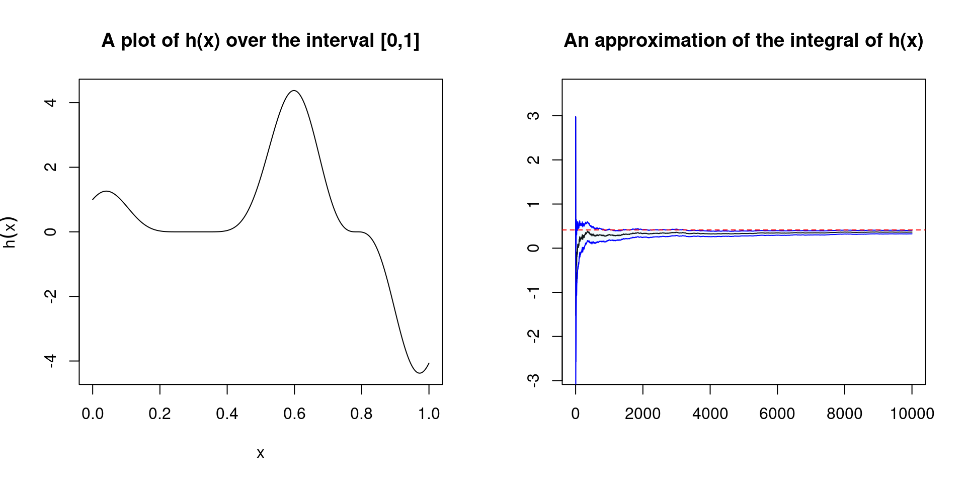
We now want to implement a plotting method which will allow us to see if the estimate has converged. We also implement a confidence bound using the asymptotic variance of the approximation \[var(\bar{h}_n) = \frac{1}{n} \int_{\mathcal{X}} (h(X) - \mathbb{E}_f[h(X)])f(x)dx\] which can be estimated using the sample \((X_1, \dots, X_n)\), by \[v_n = \frac{1}{n^2} \sum_{j=1}^n [h(x_j) - \bar{h}_n]^2.\] Using the Central Limit Theorem, for large \(n\) we have that \[\frac{\bar{h}_n - \mathbb{E}_f[h(X)])f(x)}{\sqrt{(v_n)}}\] is approximately a standard normal random variable. This then allows us to write down confidence bounds.
setMethod("plot", "monteCarloIntegration",
          function(x, ...) {
            seq_temp <- seq(x@lower_lim, x@upper_lim, length.out = 1000)
            seq_func <- x@func(seq_temp)

            r_est <- integrate(x@func, x@lower_lim, x@upper_lim)$value
            cb_lower <- x@estimates - 2*x@est_errors
            cb_upper <- x@estimates + 2*x@est_errors

            par(mfrow=c(1,2))
            plot(seq_temp, seq_func, type = 'l',
                 main = "A plot of h(x) over the interval [0,1]",
                 xlab = expression(x), ylab = expression(h(x)))
            plot(x@estimates, type = 'l',
                 ylim = c(0.8*min(cb_lower), 1.2*max(cb_upper)),
                 main = "An approximation of the integral of h(x)",
                 ylab="", xlab="")
            polygon(c(1:1e4, 1e4:1), c(cb_lower, rev(cb_upper)),
                    col = adjustcolor("skyblue", alpha.f=0.1), border = NA)
            lines(cb_lower, col = "blue")
            lines(cb_upper, col = "blue")
            abline(h = r_est, lty = 2, col = 'red')
          })
plot(integral_mc)