Vectorization
Vectorization is the process of replacing the use of loops in code, with a single operation applied elementwise to the vector. In vectorizing code, the multiple instructions running the same operation in a for loop are replaced by a single instruction which applies the operation to multiple elements in a vector.
Vectorization is much faster than using for loops in interpreted languages such as R, Matlab, and Python. To see this in practice, we will look at some examples.
We consider summing the cosine of each component of a vector.
# set the seed for reproducibility
set.seed(123)

# uses a for loop
add_cos1 <- function(x) {
  sum <- 0
  for (i in 1:length(x)) {
    sum <- sum + cos(x[i])
  }
  return(sum)
}

# uses vectorization
add_cos2 <- function(x) sum(cos(x))

x = 1:1e7
t1 <- system.time(add_cos1(x))
t2 <- system.time(add_cos2(x))
t1 ## user system elapsed
## 1.003 0.000 1.007t2## user system elapsed
## 0.364 0.075 0.440At the time of running, this provided a speedup of 2.3 times. We also note that the vectorized code is also easier to read.
High-dimensional vectorization
The example above shows that for loops are quite inefficient. It is now easy to see that nested for loops are very inefficient, and should be avoided.
There are many reasons we may want to use nested for loops. We may want to run a simulation \(n_{sim}\) times, where each simulation consists of \(n\) operations.
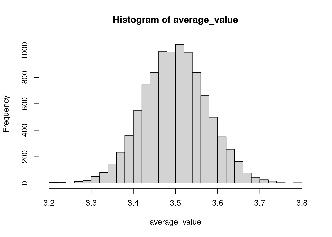
As an example, we consider the average value produced by tossing a fair six-sided die \(n=500\) times. We expect our data to center around \(\frac{1+2+3+4+5+6}{6}=3.5\). We simulate the experiment \(n_{sim} = 1000\) times.
toss_die1 <- function(nsim, n) {
  average <- numeric(nsim)
  for (i in 1:nsim) {
    counts <- numeric(n)
    for (j in 1:n) {
      counts[j] <- sample(1:6, 1)
    }
    average[i] <- mean(counts)
  }
  return(average)
}

toss_die2 <- function(nsim, n) {
  tosses <- matrix(sample(1:6, n*nsim, replace=TRUE), nrow=nsim, ncol=n)
  return(rowSums(tosses)/n)
}
We now test the runtime of the nested for loop version, and the vectorized version.
nsim <- 1000; n <- 500
t1 <- system.time(toss_die1(nsim, n)); t1
## user system elapsed
## 5.641 0.025 5.666t2 <- system.time(toss_die2(nsim, n)); t2## user system elapsed
## 0.036 0.007 0.044We see that nested for loops are very slow and should be avoided when possible. In this case the vectorized code provides a speedup of 129 times! We will use the vectorized function in the following.
nsim <- 10000; n <- 500
average_value <- toss_die2(nsim,n)
hist(average_value, breaks = 30)
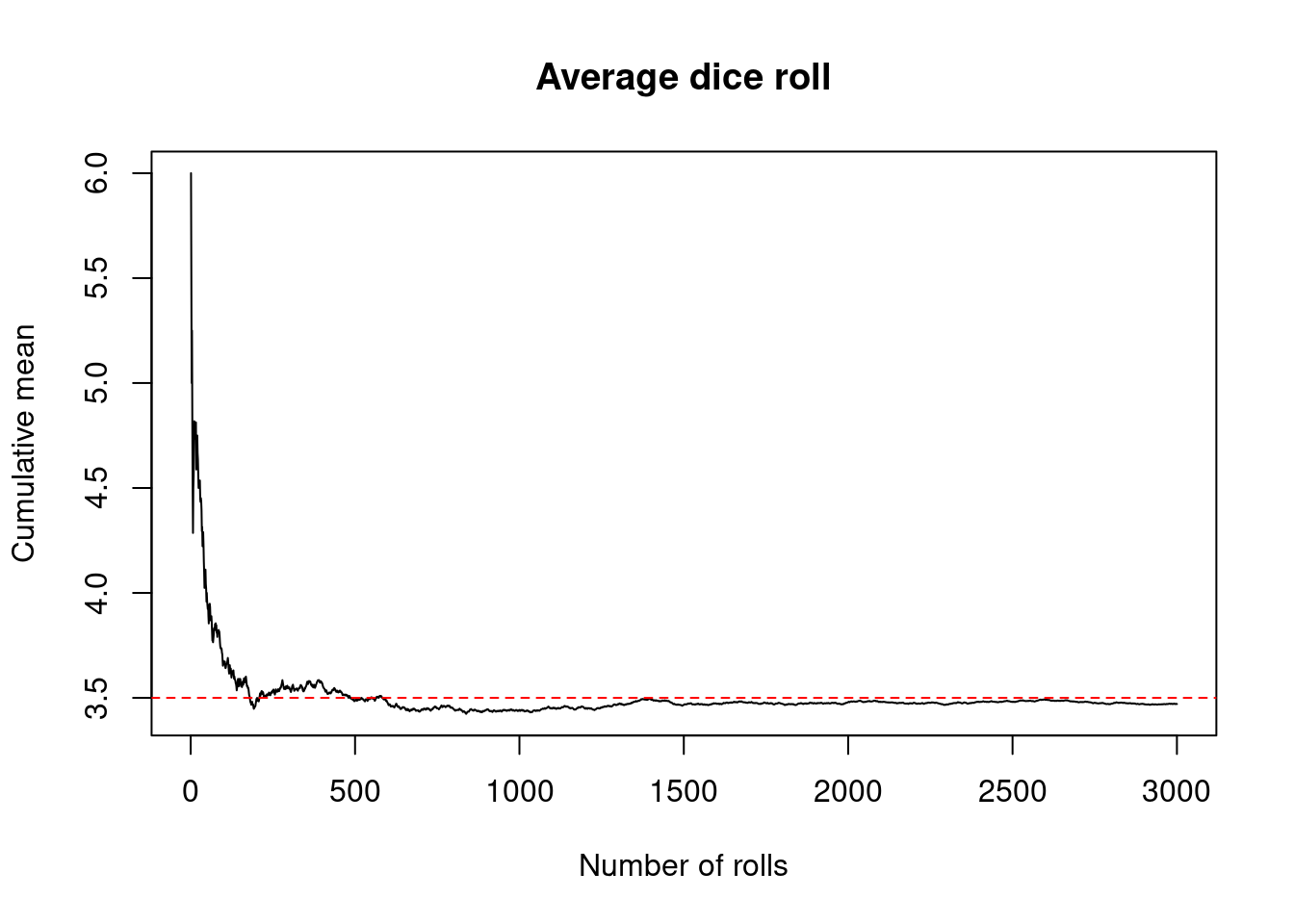
Let’s look at a demonstration of Law of Large Numbers. We plot the cumulative mean as the number of throws increases.
nsim <- 3000; n <- 1
plot(1:nsim, cumsum(toss_die2(nsim, n))/1:nsim, type = 'l',
     main='Average dice roll',
     xlab = 'Number of rolls', ylab='Cumulative mean')
abline(h=3.5, col='red', lty = 2)
The apply family
The apply family consists of apply(), lapply(), sapply(), and mapply(). These functions apply a specified function to elements in a data structure. These functions can be viewed as alternatives to for loops; they are often slower but may simplify and enhance the readability of code.
apply(X, MARGIN, FUN, ...)— This function applies a function to a vector or matrix. The MARGIN argument determines whether the function is applied over rows or columns, or both.lapply(X, FUN, ...)— This function is similar toapplybut it applies a function over a vector or list and returns a list.sapply(X, FUN, ...)— This is a wrapper function oflapplywhich simplifies the output by returning a vector, matrix, or an array when specified usingsimplify = "array".mapply(FUN, ...)— This is a multivariate version ofsapply.mapplyapplies the function FUN to the first elements of each subsequent...argument.
Examples
Below are some examples using the apply family of functions.
## apply
mat <- matrix(rep(1, 12), 3, 4) # 3x4 matrix of 1s

# apply sum to each row --- i.e. sum over columns
apply(mat, 1, sum)
## [1] 4 4 4# apply sum to each column --- i.e. sum over rows
apply(mat, 2, sum) ## [1] 3 3 3 3# apply sum to each element --- this does not do anything if FUN = sum
apply(mat, c(1,2), sum)## [,1] [,2] [,3] [,4]
## [1,] 1 1 1 1
## [2,] 1 1 1 1
## [3,] 1 1 1 1# apply our own function to each element
apply(mat, c(1,2), function(x) 2*x)## [,1] [,2] [,3] [,4]
## [1,] 2 2 2 2
## [2,] 2 2 2 2
## [3,] 2 2 2 2## lapply
vec <- rep(1,3)
lis <- list(seq = 1:4, rep = rep(1,4))
# get cosine of each element in a vector
lapply(vec, cos)## [[1]]
## [1] 0.5403023
##
## [[2]]
## [1] 0.5403023
##
## [[3]]
## [1] 0.5403023# apply cosine to list
lapply(lis, cos)## $seq
## [1] 0.5403023 -0.4161468 -0.9899925 -0.6536436
##
## $rep
## [1] 0.5403023 0.5403023 0.5403023 0.5403023## sapply
# get cosine of each element in a vector
sapply(vec, cos)## [1] 0.5403023 0.5403023 0.5403023# apply cosine to list
sapply(lis, cos)## seq rep
## [1,] 0.5403023 0.5403023
## [2,] -0.4161468 0.5403023
## [3,] -0.9899925 0.5403023
## [4,] -0.6536436 0.5403023## mapply
# sum two vectors elementwise
mapply('+', 1:3, 4:6)## [1] 5 7 9# seq(1, 5), seq(2, 5), ...
mapply(seq, 1:5, 5)## [[1]]
## [1] 1 2 3 4 5
##
## [[2]]
## [1] 2 3 4 5
##
## [[3]]
## [1] 3 4 5
##
## [[4]]
## [1] 4 5
##
## [[5]]
## [1] 5Map, Reduce, and Filter
These functions can use lambda expressions similar to the above apply family. These are short functions which are sometimes referred to as anonymous functions, as they are not assigned to a variable. Lambda expressions allow us to produce quite complicated functionality in one line.
Below is a quick summary of the functions introduced in this section:
Map— This function maps a function to every element in a vector.Reduce— This function performs a function on pairs of elements in a vector, iteratively, and returns a single number.Filter— Tests every element in a vector and only returns those that satisfy the condition.
Examples
Below are some examples demonstrating the above functions.
vec <- 1:3

# Map cosine to every element in a vector
Map(cos, vec)
## [[1]]
## [1] 0.5403023
##
## [[2]]
## [1] -0.4161468
##
## [[3]]
## [1] -0.9899925# Reduce
Reduce(function(x, y) x + 2*y, vec)## [1] 11# Filter
Filter(function(x) x %% 3 == 0, vec) ## [1] 3Parallel computing
Parallelization is the process of using multiple CPU cores at the same time, to solve different parts of a problem. Often when working on large computational problems, we will encounter a bottleneck. We may encounter a
- CPU-bound: Our computations take too much CPU time.
- Memory-bound: Our computations use too much memory.
- I/O bound: It takes too long to read/write from disk.
Parallel computing helps us overcome CPU bounds by working with more than one core at a time. This means that if our computer has four physical cores, then we can distribute our computation across four cores. In theory, this would speed up our computation by four times but it is not the case in practice due to the other bounds described above. Part of being a good R programmer is being able to write fast and efficient code.
Parallelize using mclapply
mclapply is a multi-core version of lapply.
library(parallel)
library(doParallel)
## Loading required package: foreach## Loading required package: iterators# detect cores
detectCores()## [1] 8# demonstrate that distributing over 4 cores does not provide speed up of 4 times
system.time(lapply(1:8, function(x) Sys.sleep(0.5))) # 4 seconds## user system elapsed
## 0.003 0.000 4.007system.time(mclapply(1:8, function(x) Sys.sleep(0.5), mc.cores=4)) # expect 1 second## user system elapsed
## 0.009 0.033 1.025Parallelize using foreach
foreach seems a little like a for loop. However foreach uses binary operators %do% and %dopar%, and also returns a list as output. It’s useful to use foreach with %do% to evaluate an expression sequentially and store all outputs in a data struture — by default this is a list but the behavior can be changed using the argument .combine.
library(foreach)

# run sequentially using %do%
foreach(i=1:3) %do% {i*i}
## [[1]]
## [1] 1
##
## [[2]]
## [1] 4
##
## [[3]]
## [1] 9# change output to vector
foreach(i=1:3, .combine="c") %do% {i*i}## [1] 1 4 9The above functions use the operator %do% and therefore run sequentially. If we simply replace the operator with %dopar% R will run the computations in parallel. The above computations are so simple that it’s probably not worth implementing them in parallel. Let’s look at a little example using Markov chain Monte Carlo, in which we may want to run multiple chains to test for pseudo-convergence. All of the parallelization is in the simulate.chains function. Note that in order to run the computations in parallel we must register the parallel backend using registerDoParallel(<cores>) before foreach. When we are finished we should run stopImplicitCluster().
# returns the transition kernel P(x)
make.metropolis.hastings.kernel <- function(pi, Q) {
  q <- Q$density
  P <- function(x) {
      z <- Q$sample(x)
      alpha <- min(1, pi(z) * q(z, x) / pi(x) / q(x, z))
      if(runif(1) < alpha) {
        return(z)
      } else {
        return(x)
      }
  }
  return(P)
}

make.normal.proposal <- function(sigma) {
  Q <- list()
  Q$sample <- function(x) {
    return(rnorm(length(x), x, sigma))
  }
  Q$density <- function(x, z) {
    return(dnorm(z, x, sigma))
  }
  return(Q)
}

simulate.chains <- function(P, x0, n, n.chains, n.cores = 4) {
  # parallelize chains
  registerDoParallel(n.cores)
  simulations <- foreach(i=1:n.chains, .combine="rbind") %dopar% {
    x <- x0[i]
    foreach(i=1:n, .combine="c") %do% {P(x)}
  }
  stopImplicitCluster()
  return(simulations)
}
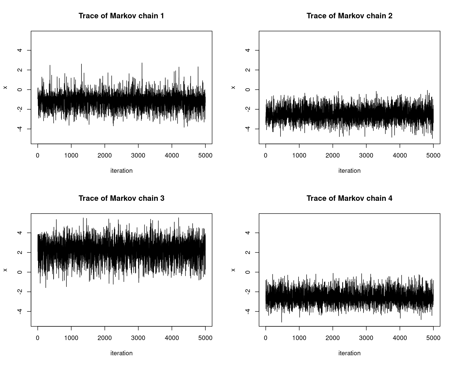
Below we sample from a mixture distribution: The weighted mixture of two normal distributions \({Z \sim 0.6X + 0.4Y}\), where \(X \sim N(-2,1)\), \(Y \sim N(5, 2^2)\). We use a \(N(0,1)\) proposal distribution. We will run \(4\) chains in parallel and test for pseudo-convergence by looking at the trace of the chains. Each chain is initialized using a \(U[-10,10]\) distribution.
# generate markov chain using MH algorithm
# target: mixture of two normals
n <- 5e3; set.seed(123)
target <- function(x) {0.6*dnorm(x, -2, 1) + 0.4*dnorm(x, 5, 2)}
xs <- simulate.chains(make.metropolis.hastings.kernel(target, make.normal.proposal(1)),
                      runif(4,-10,10), n, 4)

# setup plot space
par(mfrow=c(2,2))

# plot the chains
ylimits <- c(min(xs), max(xs))
for(i in 1:4){
  plot(1:n, xs[i,], type = 'l', xlab="iteration", ylim=ylimits,
       ylab="x", main=paste0("Trace of Markov chain ", i))
}
We see that the traces do not converge to the same distribution! This tells us that the chains are not fully exploring the state space and thus we must adjust our proposal distribution.