Reproducible research

Reproducible research refers to the idea that given an academic paper and the author’s raw data, anyone interested can carry out the exact same computations and produce the same result which was published.

A large portion of academic research is not reproducible. The scientific method revolves around making assumptions, producing hypotheses, and rigorously detailing how a conclusion is produced. Very little computationally-intensive scientific research adequately explains the modelling choices that were made, and so their claims cannot be verified. Some researchers focus on developing different models and architectures which excel at certain tasks, and we are often presented with the model’s prediction/classification performance on an array of datasets. However in producing these results various choices have been made which may not have been adequately explained — we may question how the data was split into train/test sets, how the model’s hyperparameters were chosen, how we can know that the model hasn’t simply overfit the data, etc. Given such complicated experiments, the original authors themselves may not be able to replicate their findings exactly. In some fields such as deep learning, verifying the performance of state-of-the-art (SOTA) algorithms/architectures by training a model from scratch becomes impossible due to the large amount of resources required to re-run experiments. For example, Google has open-sourced the code for its SOTA language model BERT, but the pre-trained model is rumored to have cost $30,000 to train. It would not be possible to re-train BERT without extensive resources. We can of course verify the performance of BERT on an unseen dataset, but we cannot reproduce BERT.

Historically, producing reproducible research has been difficult as it would be very hard to perfectly replicate the original computing environment. A lot of research is also quite interactive. When analyzing data we frequently produce visualizations and test our hypotheses interactively, and we often do not store all of the code we have used. The wealth of tools available to us today make these reasons redundant. Analyses are often carried out with high-level programming languages such as R and Python, which produce the same output when run on different hardware with different operation systems. Package management systems record the computational environment to ensure it can be replicated, and version control systems such as git rigorously keep track of all changes in code. Code can easily be pushed to github and made available to the public.

There are some valid reasons why researchers may not publish their code. Due to the nature of some fields such as healthcare and defense, raw data simply cannot be shared. It is also possible that personal data is being used and for reproducibility data is sometimes released in an anonymized form. Data anonymization is very difficult to do correctly — the Netflix Prize is an infamous example in which supposedly anonymous Netflix data was de-anonymized. In 2019 OpenAI published a blog post and paper claiming the SOTA performance of their language model GPT-2, but they chose not to publish the full model, the training dataset, and the training code, as they believed it to be too dangerous. Instead they released a much smaller version of GPT-2 and proposed a ‘staged’ release system in which they incrementally released larger versions of GPT-2.

When the Royal Society was founded in 1660, its motto was chosen to be Nullius in verba — Latin for “on the word of no one” or “take nobody’s word for it”. Reproducibility has long been something to strive for. In recent years we have seen the replication crisis appearing in different fields. Psychology has begun a large-scale effort to replicate significant and historical results. Brian Nosek of the Center for Open Science led sixty labs in thirty-six countries in recreating twenty-eight experiments (combined sample sizes were sixty-two times larger than the original experiment on average). Only fourteen of twenty-eight results were successfully replicated.

Literate programming

Donald Knuth introduced the concept of literate programming in 1984. The idea is that a computer program or analysis should consist of an explanation of its logic in a natural language such as English, accompanied by snippets of code which carry out the proposed logic. Knuth said that “Instead of imagining that our main task is to instruct a computer what to do, let us concentrate rather on explaining to human beings what we want a computer to do.”.

In practice, we produce a document explaining what a program does in addition to code that can be executed. RMarkdown makes it easy to create documents that ensure code and documentation are consistent with one another, and allows us to emphasize the readability of the document. RMarkdown greatly improves upon simply commenting throughout an R script when producing high-level analyses. However, when working low-level functionality an R script with accompanying documentation is often preferred.

Example

Here we look at a simple example of literate programming.

Let’s import some data. We will look at Bristol weather data which has been compiled from multiple sources. The source of this .txt file can be found here.

library(readr)
bristoltemps <- read_csv("../data/bristoltemps.txt")

## Rows: 1991 Columns: 3
## ── Column specification ────────────────────────────────────────────────────────
## Delimiter: ","
## dbl (3): Year, Month, Temperature
## 
## ℹ Use `spec()` to retrieve the full column specification for this data.
## ℹ Specify the column types or set `show_col_types = FALSE` to quiet this message.

head(bristoltemps)

## # A tibble: 6 × 3
##    Year Month Temperature
##   <dbl> <dbl>       <dbl>
## 1  1853     1           5
## 2  1853     2           1
## 3  1853     3           3
## 4  1853     4           7
## 5  1853     5          11
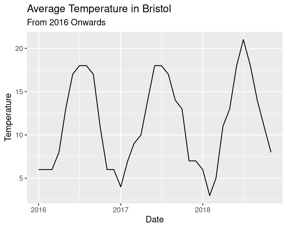
## 6  1853     6          13

We will use the tidyverse to quickly produce some plots. It may be interesting to view the temperature over a few years to view the periodicity.

# add a date column in the format yyyy-mm-dd
bristoltemps <- bristoltemps %>% 
  mutate("Date" = as.POSIXct(paste0(Year, "-", Month, "-01")))

# create a plot from 2016-2018
bristoltemps %>%
  filter(Year >= 2016) %>%
  ggplot(aes(x = Date, y=Temperature)) +
  geom_line() +
  labs(title = "Average Temperature in Bristol", 
       subtitle = "From 2016 Onwards")

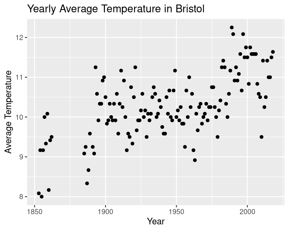
We may also be interested in the change in the annual temperature in Bristol. Let’s produce a plot of that.

# compute average temperature per year and plot over time
bristoltemps %>%
  group_by(Year) %>%
  summarise("Average Temperature" = mean(Temperature)) %>%
  ggplot(aes(x = Year, y = `Average Temperature`)) +
  geom_point() +
  labs(title = "Yearly Average Temperature in Bristol")

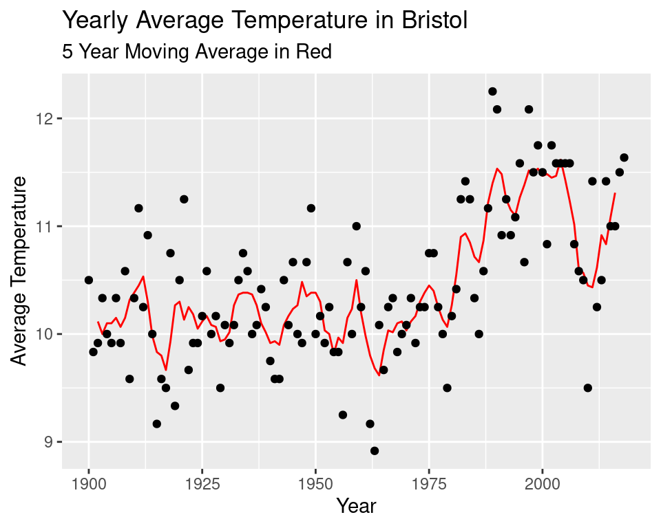
We seem to be missing some data somewhere between 1850 and 1900. So we will only consider data from the year 1900 onwards. The erratic nature of the data makes it difficult to see a pattern so we will implement a 5 year moving average.

# function that returns the moving average over n values
ma <- function(x, n) {
  return(stats::filter(x, rep(1/n, n), sides=2))
}

# produce a plot with a 5 year average over the data
bristoltemps %>%
  filter(Year >= 1900) %>%
  group_by(Year) %>%
  summarise("Average Temperature" = mean(Temperature)) %>%
  ggplot(aes(x = Year, y = ma(`Average Temperature`, 5))) +
  geom_line(col="red") +
  geom_point(aes(x = Year, y = `Average Temperature`)) +
  labs(title = "Yearly Average Temperature in Bristol",
       subtitle = "5 Year Moving Average in Red",
       y = "Average Temperature")

## Don't know how to automatically pick scale for object of type ts. Defaulting to continuous.

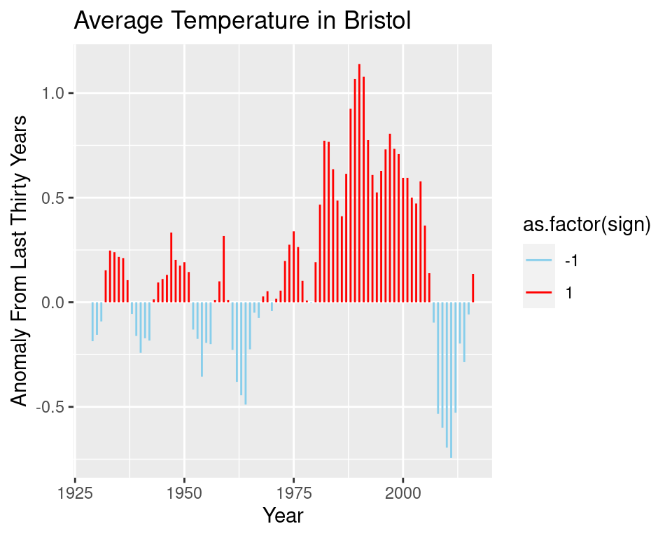
It may be interesting to see the change in temperature relative to an average of the last \(30\) years. We redefine our function ma to allow us to average over the past values, and produce a new plot of the differences between the temperature in year \(x\) and the average over the last \(30\) years.

Note that below we actually compute a moving average over 5 yearly temperatures, and compare this to the average temperature of the last 30 years. This is done because the data is a combination of different datasets from various weather stations in Bristol. The measuring apparatus will change over time.

# function that returns the average over n values
ma <- function(x, n, sides) {
  return(stats::filter(x, rep(1/n, n), sides=sides))
}

# produce plot
bristoltemps %>%
  filter(Year >= 1900) %>%
  group_by(Year) %>%
  summarise("Average Temperature" = mean(Temperature)) %>%
  mutate(avg_last_thirty_years = ma(`Average Temperature`, 30, sides=1)) %>%
  mutate(diff = ma(`Average Temperature`, 5, sides=2) - avg_last_thirty_years,
         sign = sign(diff)) %>%
  na.omit() %>% 
  ggplot(aes(x = Year, y = diff)) +
  geom_segment(aes(xend = Year, col = as.factor(sign)), yend= 0) +
  scale_colour_manual(values = c("skyblue", "red")) +
  labs(title = "Average Temperature in Bristol",
       y = "Anomaly From Last Thirty Years")