Numerical Integration
Quadrature
“Quadrature rules” are integral approximations which use a finite number of evaluations of the function. All of the quadrature rules below approximate a function using interpolating polynomials.
We will first look at some key ideas in numerical integration by approximating definite integrals over a finite interval. We will then extend these ideas to semi-infinite and infinite intervals. We will also consider multiple integrals.
In practice we can use Rs integrate function for one-dimensional integrals, and the cubature package for multiple integrals.
Polynomial Interpolation
We consider approximating a continuous function \(f\) on \([a,b]\) (this can be written \(f \in C^0([a,b])\)), using a polynomial function \(p\). We know how to compute integrals of polynomials exactly, and so if \(p\) is a good approximation of our integrand then we can compute an accurate approximation to the integral. The Weierstrass Approximation Theorem provides a high-level motivation.
Weierstrass Approximation Theorem. Let \(f \in C^0([a,b])\). There exists a sequence of polynomials \((p_n)\) that converges uniformly to \(f\) on \([a,b]\). That is, \[ \|f - p_n\|_\infty = \max_{x \in [a,b]} |f(x) - p_n(x)| \rightarrow 0.\]
The above theorem suggests that for any given tolerance, we can find a polynomial which approximates a function \(f \in C^0([a,b])\) up to said tolerance. The Weierstrass theorem tells us that such polynomials exist, but it does not tell us how to find them. The real difficulty lies in constructing such polynomials in a computationally-efficient manner without a strong knowledge of the function \(f\).
Lagrange polynomials
We can approximate a function \(f\) by using an interpolating polynomial with \(k\) points \(\{x_i, f(x_i)\}_{i=1}^n\). The interpolating polynomial produced is unique, has at most \(k-1\) degree, and can be written as a Lagrange polynomial: \[p_{k-1}(x) := \sum_{i=1}^k \ell_i(x) f(x_i),\] where the Lagrange basis polynomials are \[\ell_i(x) = \prod_{j=1, j\neq i}^p \frac{x - x_j}{x_i - x_j}, \quad i \in \{1, \dots, k\}.\]
Below is code implementing interpolating polynomials. For a polynomial with degree \(3\) we can produce the polynomial approximations for \(k \in \{2,3,4\}\) and for specific choices of \(x_1, \dots, x_4\).
construct.interpolating.polynomial <- function(f, xs) {
  k <- length(xs)
  fxs <- f(xs)
  p <- function(x) {
    value <- 0
    for (i in 1:k) {
      fi <- fxs[i]
      zs <- xs[setdiff(1:k,i)]
      li <- prod((x-zs)/(xs[i]-zs))
      value <- value + fi*li
    }
    return(value)
  }
  return(p)
}

plot.polynomial.approximation <- function(f, xs, a, b) {
  p <- construct.interpolating.polynomial(f, xs)
  vs <- seq(a, b, length.out=500)
  plot(vs, f(vs), type='l', xlab="x", ylab="black: f(x), red: p(x)")
  points(xs, f(xs), pch=20)
  lines(vs, vapply(vs, p, 0), col="red")
}

a <- -4
b <- 4

f <- function(x) {
  return(-x^3 + 3*x^2 - 4*x + 1)
}

par(mfrow=c(1,3))
plot.polynomial.approximation(f, c(-2, 2), a, b)
plot.polynomial.approximation(f, c(-2,0,2), a, b)
plot.polynomial.approximation(f, c(-2, 0, 2, 4), a, b)
Interpolation Error and Convergence
Clearly we can approximate a polynomial using interpolating polynomials for a \(k\) which is large enough. However, we are often interested in approximating functions which are not polynomials.
Interpolation Error Theorem. Let \(f \in C^k[a,b]\), and \(p_{k-1}\) be the polynomial interpolating \(f\) at the \(k\) points \(x_1, \dots, x_k\). Then for any \(x \in [a,b]\) there exists \(\xi \in (a,b)\) such that \[f(x) - p_{k-1}(x) = \frac{1}{k!}f^{(k)}(\xi) \prod_{i=1}^k (x - x_i).\] The above theorem looks promising, but it does not tell us how to choose our interpolating polynomials such that they converge uniformly (or even pointwise) to \(f\). The theorem tells us that one way of minimizing the error is to choose the interpolation points such that the product \(|\prod_{i=1}^k (x - x_k)|\) is as small as possible. The Chebyshev interpolation points detailed below do this.
We know that there exists a sequence of interpolation points that provide us with uniform convergence.
Theorem. Let \(f \in C^0[a,b]\). There exists a sequence of sets of interpolation points \(X_1, X_2, \dots\) such that the corresponding sequence of interpolating polynomials converges uniformly to \(f\) on \([a,b]\).
The above tells us that given a function \(f\), it is indeed possible to find a sequence of sets of interpolating points which produce a sequence of interpolating polynomials that converge uniformly to \(f\). We may then wonder if there is a universal sequence of sets of interpolating points that provide us with uniform convergence to any function \(f\). This is not possible, as for any fixed sequence of sets we can find a function \(f\) for which our sequence of interpolating polynomials diverges.
Theorem. For any fixed sequence of sets of interpolation points there exists a continuous function \(f\in C^0[a,b]\) for which the sequence of interpolating polynomials diverges on \([a,b]\).
Example: Consider the sequence of interpolating points \(X_k\) to be the set of \(k\) uniformly spaced points including a, and b if \(k>1\).
This is a particularly bad way to produce sets of interpolation points as uniform convergence is not guaranteed — even for infinitely differentiable functions. There are of course functions which these interpolation points work well for, as seen below.
construct.uniform.point.set <- function(a, b, k) {
  if (k==1) return(a)
  return(seq(a, b, length.out=k))
}

a <- 1
b <- 2
plot.polynomial.approximation(log, construct.uniform.point.set(a, b, 10), a, b)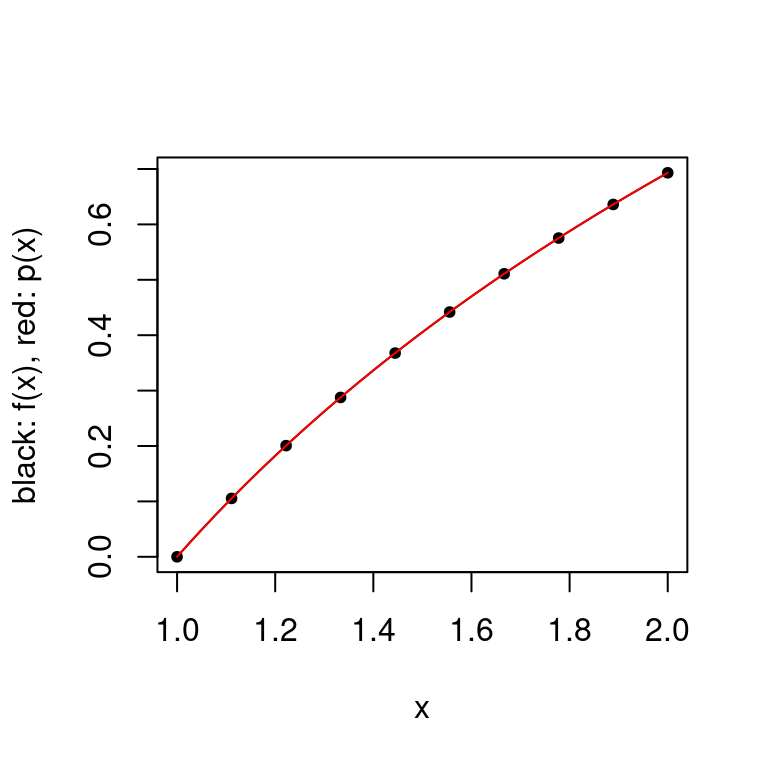
Below is a plot of the Runge function defined by \(f(x) = \frac{1}{1+x^2}\) over the interval \([-5,5]\). We see that the interpolation error \(\|f-p_n\|_\infty\) grows without bound as \(n \rightarrow \infty\).
Below we look at the polynomial interpolation of the Runge function \(f(x) = \frac{1}{1+x^2}\), over the interval \([-5,5]\).
a <- -5
b <- 5
f <- function(x) return(1/(1+x^2))
plot.polynomial.approximation(f, construct.uniform.point.set(a,b,50), a, b)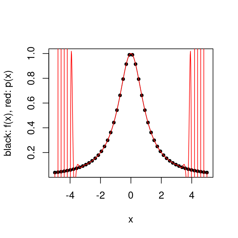
Note that this does not contradict the Interpolation Error Theorem as the maximum of the \(k\)’th derivative of the Runge function grows quickly with \(k\). As this outweighs the decreasing product term, the interpolation error grows without bound as \(k \rightarrow \infty\).
We can also look at the function \(f(x) = |x|\) over \([-1,1]\). We see that the interpolating polynomial oscillates wildly for large \(k\).
a <- -1
b <- 1
par(mfrow=c(1,3))
plot.polynomial.approximation(abs, construct.uniform.point.set(a,b,50), a, b)
plot.polynomial.approximation(abs, construct.uniform.point.set(a,b,100), a, b)
plot.polynomial.approximation(abs, construct.uniform.point.set(a,b,200), a, b)
Note once again that this does not contradict the Interpolation Error Theorem as the function \(f(x)\) is not differentiable at \(0\).
As mentioned above, we can avoid this problem by minimizing the interpolation error by minimizing the product term. If we minimize the maximum absolute value of the product term, we can derive the Chebyshev interpolation points. For any given \(k\), we have the points \[\cos\left(\frac{2i-1}{2k}\pi\right), \quad i \in \{1, \dots, k\},\] and the absolute value of the product term is then bounded above by \(2^{1-k}\)
These points clearly do not minimize the overall error.
construct.chebyshev.point.set <- function(k) {
  return(cos((2*(1:k)-1)/2/k*pi))
}

# visualize the Chebyshev points
chebyshev.visalization <- function(k){
  df <- data.frame(k = numeric(), points = list())
  for(i in 1:k){
    df <- rbind(df, data.frame(k=i, points = construct.chebyshev.point.set(i)))
  }
  ggplot(df, aes(color=k, x = points, y = k)) +
    geom_point(aes(color=k)) +
    labs(y="number of points k", xlab="")
}

# produce visualization
chebyshev.visalization(50)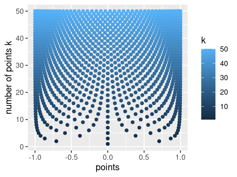
Above we clearly see that as our number of points \(k\) increases, the points tend to cluster around \(-1\), and \(1\). We can use the Chebyshev interpolation points as seen below.
plot.polynomial.approximation(f, construct.chebyshev.point.set(50), a, b)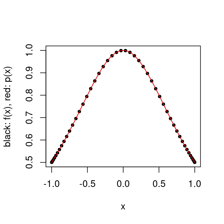
plot.polynomial.approximation(abs, construct.chebyshev.point.set(50), a, b)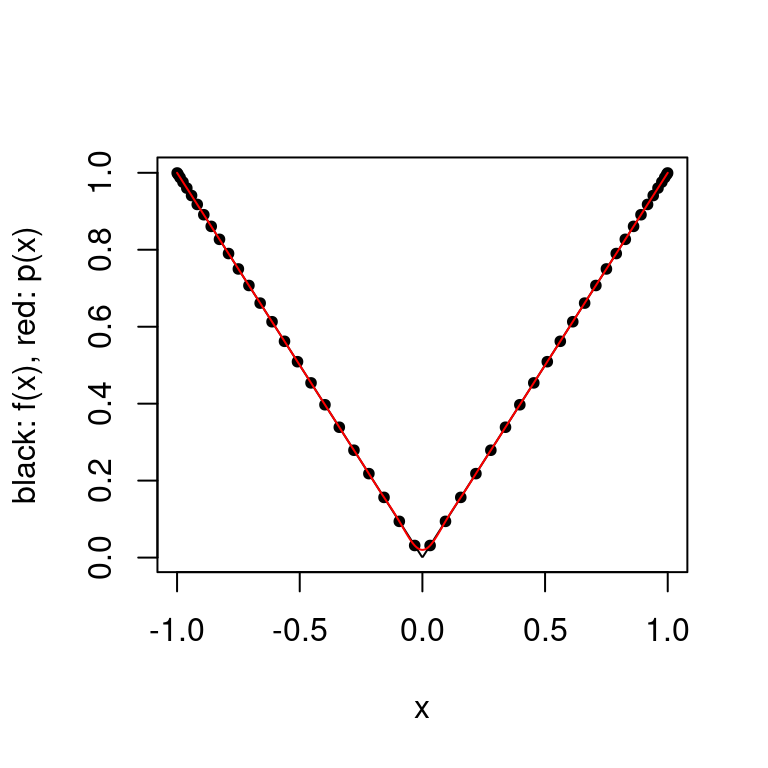
There is a large improvement in the error as the approximation no longer oscillates. As mentioned in the theorem above, there exist functions \(f\) for which the interpolating polynomials with the Chebyshev interpolating points diverge.
Composite Polynomial Interpolation
Another way to approximate a function is to use different polynomials over subintervals of the domain. This results in a piecewise polynomial approximation which is not necessarily continuous, but can be made to be.
Other Polynomial Interpolation Schemes
There are many other schemes that we may use to approximate a function. We may use Hermite interpolation which fits a polynomial using evaluations of \(f\) and evaluations of the derivatives of \(f\). If we ensure that the derivatives at the boundaries of the subintervals are equal then the resulting approximation will have a certain number of continuous derivatives. This idea is known as spline interpolation, and is often preferred to polynomial interpolation as it avoids the problem of Runge’s phenomenon demonstrated above. Spline interpolation also produces a small interpolation error even when using low degree polynomials.
Below is an implementation of natural cubic spline interpolation. For a set of interpolation points \(\{x_i\}_{i=1}^n\), a cubic spline fits a polynomial of at most degree \(3\) between each pair of interpolating points. Hence for a set of \(n\) interpolation points, \(n-1\) splines are produced to approximate the function. A set of constraints are placed upon the values these splines can take, which ensure that the spline is continuous over the interval. A natural cubic spline has degree \(3\) with continuity \(C^2\), and has the general form \[S_j(x) = a_j + b_j(x - x_j) + c_j(x - x_j)^2 + d_j(x - x_j)^3, \quad j = 0, \dots, n-1\] for which the individual splines must satisfy \[\begin{align*} &S_i(x_i) &&= y_i \qquad &&i = 0, \dots, n-1\\ &S_{i-1}(x_i) &&= y_i &&i = 1, \dots, n\\ &S'_{i}(x_i) &&= S'_{i-1}(x_i) &&i = 1, \dots, n-1 \\ &S''_{i}(x_i) &&= S''_{i-1}(x_i) &&i = 1, \dots, n-1 \\ &S''_{0}(x_0) &&= S''_{n-1}(x_{n-1}) = 0 &&i = 1, \dots, n-1 \\ \end{align*}\]
An implementation can be seen below.
# compute spline parameters
create.spline.params <- function(f, xs) {
  n <- length(xs) - 1
  fxs <- f(xs)
  b <- d <- rep(0,n)
  h <- diff(xs)
  hlag2 <- diff(xs, lag=2)
  alpha <- 3/h[-1]*diff(fxs)[-1] - 3/h[-n]*diff(fxs)[-n]
  c <- l <- mu <- z <- rep(0,n+1)
  l[1] <- 1; mu[1] <- z[1] <- 0
  for (i in 2:(n)) {
    l[i] <- 2*hlag2[i-1] - h[i-1]*mu[i-1]
    mu[i] <- h[i]/l[i]
    z[i] <- (alpha[i-1]-h[i-1]*z[i-1])/l[i]
  }
  l[n+1] <- 1; z[n+1] <- c[n+1] <- 0
  for (j in n:1) {
    c[j] <- z[j] - mu[j]*c[j+1]
    b[j] <- (fxs[j+1] - fxs[j])/h[j] - h[j]*(c[j+1] + 2*c[j])/3
    d[j] <- (c[j+1]-c[j])/(3*h[j])
  }
  return(list(a=fxs, b = b, c = c, d = d))
}

# given parameters and the interval, return appropriate spline function
# this is needed as for n interpolation points, n-1 splines are produced
construct.spline <- function(a, b, c, d, i, xs) {
  return(function(x) a[i] + b[i]*(x - xs[i]) + c[i]*(x - xs[i])^2 + d[i]*(x - xs[i])^3)
}

# given x and interpolation points, return spline index
get.spline.subinterval <- function(x, xs){
  n <- length(xs-1)
  for(i in 1:n) {
    if (between(x, xs[i], xs[i+1])) return(i)
  }
}

# produce and plot the spline approximation for a function f and interpolation points xs
plot.cubic.splines.approximation <- function(f, xs){
  par <- create.spline.params(f, xs)
  spline <- function(x) construct.spline(par$a, par$b, par$c, par$d,
                                         get.spline.subinterval(x, xs), xs)(x)
  vs <- seq(min(xs), max(xs), length.out=500)
  plot(vs, f(vs), type='l', xlab="x", ylab="black: f(x), red: p(x)")
  abline(v=xs, col = "grey")
  lines(vs, f(vs))
  lines(vs, vapply(vs, spline, 0), col="red")
  points(xs, f(xs), pch=20, col="blue")
}
par(mfrow=c(1,2))
plot.cubic.splines.approximation(sin, seq(0,4*pi, length.out=4))
plot.cubic.splines.approximation(sin, seq(0,4*pi, length.out=12))
We see that our approximation is not very accurate when we have a small set of interpolation points, but we can approximate the \(\sin\) function impressively well with only \(12\) interpolation points and with polynomials of at most degree \(3\)!
plot.cubic.splines.approximation(function(x) abs(x), seq(-1,1, length.out=16))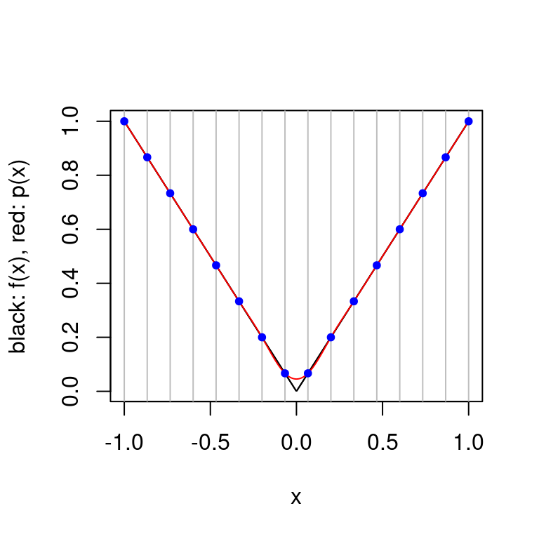 Splines avoid the oscillating approximation phenomenon which occurs with polynomial interpolation. For the function \(f(x)=|x|\), the spline method seems to work better than the interpolating polynomial approach but it is not possible for the approximation to capture the true behavior of \(f(x)\) around \(x=0\). This is because \(f\) is not continuous at this point and an explicit requirement on the natural cubic spline is that it is continuous.
par(mfrow=c(1,2))
plot.cubic.splines.approximation(function(x) 1/(1+25*x^2), seq(-5,5, length.out=6))
plot.cubic.splines.approximation(function(x) 1/(1+25*x^2), seq(-5,5, length.out=16))
plot.cubic.splines.approximation(function(x) 1/(1+25*x^2), seq(-5,5, length.out=45))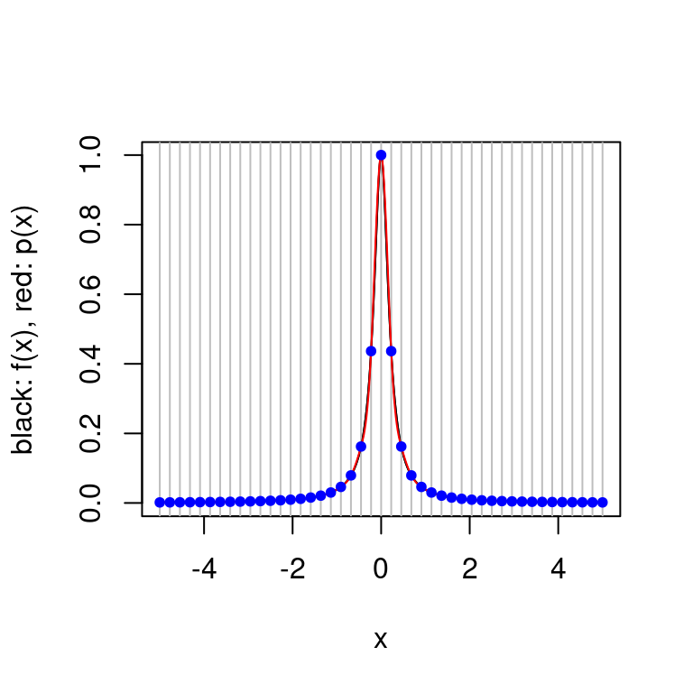 Above we see that Runge’s phenomenon does not occur for splines, but it is hard to produce a good approximation to Runge’s function for a small number of interpolation points. Of course small has little meaning — in this case it is very easy to evaluate Runge’s function for a large number of points, for other functions this may not be true.
Monte Carlo Integration
The quadrature rules introduced above give excellent rates of convergence (in terms of computational cost) for low-dimensional problems. Their costs quickly become too expensive for high-dimensional problems. For such problems, a better approach is to use Monte Carlo algorithms.
Let \((X, \mathcal{X})\) be a measurable space. We have a target probability measure \(\pi:\mathcal{X} \rightarrow [0,1]\) and we would like to approximate the quantity \[\pi(f) := \int_X f(x) \pi(dx),\] where \(f \in L_1(X, \pi) = \{f:\pi(|x|)<\infty\}\). I.e. \(\pi(f)\) is the expectation of \(f(X)\) when \(X \sim \pi\).
Monte Carlo with IID Random Variables
Classical Monte Carlo is a natural method for integral approximation. We can motivate its use at a high level using the Law of Large Numbers. Recall that our aim is to approximate the quantity \(\pi(f)\); below we reduce this problem to the problem of simulating random variables with distribution \(\pi\).
Fundamental Results
Theorem(SLLN): Let \((X_n)_{n\geq1}\) be a sequence of iid random variables with distribution \(\mu\). Define the quantity \[S_n(f) := \sum_{i=1}^n f(X_i)\] for \(f \in L_1(X, \mu)\). Then \[\lim_{n \rightarrow \infty} \frac{1}{n}S_n(f) = \mu(f),\] almost surely.
The random variable \(n^{-1}S_n(f)\) is a Monte Carlo approximation of \(\mu(f)\). The probabilistic convergence result does not tell us about the variance of the approximation for finite \(n\), so we compute the variance of the approximation and appeal to the Central Limit Theorem.
Proposition(Variance): Let \((X_n)_n\geq1\) and \(S_n(f)\) be as defined in the SLLN, where \(f\in L_2(X, \mu)\). Then \[Var[n^{-1}S_n(f)] = \frac{\mu(f^2) - \mu(f)^2}{n}.\]
Theorem(CLT): Let \((X_n)_n\geq1\) and \(S_n(f)\) be as defined in the SLLN, where \(f\in L_2(X, \mu)\). Then \[n^{1/2}\{n^{-1}S_n(f) - \mu(f)\} \xrightarrow[]{L} X \sim N(0, \mu(\bar{f}^2)),\] where \(\bar{f} = f - \mu(f)\).
Sampling
The SLLN and CLT which justify our approximations above rely on us being able to simulate random variables from our target distribution \(\mu=\pi\). This is the main difficulty in Monte Carlo methods — we often have limited knowledge of \(\pi\).
Classical Monte Carlo methods differ in the way that they generate samples from \(\pi\). Some very well-known Monte Carlo algorithms are:
- Rejection sampling
- Importance sampling
- Self-normalized importance sampling
Markov Chain Monte Carlo (MCMC)
Markov chain Monte Carlo (MCMC) methods are a development of the standard Monte Carlo techniques. These methods allow us to sample from a probability distribution by constructing a Markov chain as opposed to sampling independent random variables.
Fundamental Results
Theorem(LLN for Markov chains): Suppose that \(\mathbf{X}=(X_n)_{n\geq0}\) is a time-homogeneous, positive Harris Markov chain with invariant probability measure \(\pi\). Then for any \(f \in L_1(X, \pi)\), \[\lim_{n \rightarrow \infty} \frac{1}{n} S_n(f) = \pi(f),\] almost surely for any initial distribution for \(X_0\).
Similar to classical Monte Carlo, there also exist Central Limit Theorems for Markov chains such as the following
Theorem(A CLT for geometrically ergodic Markov chains): Assume that \(\mathbf{X}\) is time-homogeneous, positive Harris and geometrically ergodic with invariant probability measure \(\pi\), and that \(\pi(|f|^{2+\delta})<\infty\) for some \(\delta>0\). Then \[n^{1/2} \{ n^{-1} S_{n}(f) - \pi(f) \} \overset{L}{\to} N(0,\sigma^{2}(f))\] as \(n\rightarrow\infty\), where \(\bar{f}=f-\pi(f)\) and \[\sigma^{2}(f)=\mathbb{E}_{\pi}\left[\bar{f}(X_{0})^{2}\right]+2\sum_{k=1}^{\infty}\mathbb{E}_{\pi}\left[\bar{f}(X_{0})\bar{f}(X_{k})\right]<\infty.\]
The Law of Large Numbers and Central Limit Theorem results for Markov chains tell us that we are justified in using Markov chains to produce samples from a distribution, as long as certain conditions are met (e.g. time-homoegeneity, chain is positive Harris recurrent, etc.). Our aim is therefore to produce transition kernels and thus Markov chains which satisfy these conditions.
Metropolis-Hastings
Metropolis-Hastings (MH) transition kernels are perhaps the most used method of constructing Markov chains. The MH algorithm is as follows:
Suppose we want to sample from a target distribution \(\pi\), which has a density with respect to (w.r.t) some measure \(\lambda\). We specify a proposal Markov kernel \(Q\) admitting density \(q\) w.r.t \(\lambda\), i.e. \(Q(x, dz) = q(x, dz) \lambda (dz)\).
In order to sample from \(\pi\), we simulate according to the transition kernel \(P_{MH}(x, \cdot)\).
Initialize: Set \(X_1 = x_1\).
For \(t = 2, \dots\)
2a. Sample a proposal \(Z \sim Q(x_t, \cdot)\).
2b. Accept proposal \(Z\) with the acceptance probability \(\alpha_{MH}(x_t, Z)\), where \[\alpha_{MH}(x, z) := \min\left(1, \frac{\pi(z) q(z, x)}{\pi(x) q(x, z)}\right),\] otherwise, output \(x_t\).
Note that given the acceptance probability specified by the MH algorithm, we only need to know the density \(\pi\) up to a normalizing constant. Also, in the case that a symmetric proposal (i.e. \(q(x, y) = q(y, x)\) for all \(x, y\)) is specified, the MH update becomes the Metropolis update.
Below is an implementation of the Metropolis-Hastings algorithm.
# returns the transition kernel P(x)
make.metropolis.hastings.kernel <- function(pi, Q) {
  q <- Q$density
  P <- function(x) {
      z <- Q$sample(x)
      alpha <- min(1, pi(z) * q(z, x) / pi(x) / q(x, z))
      if(runif(1) < alpha) {
        return(z)
      } else {
        return(x)
      }
  }
  return(P)
}

make.normal.proposal <- function(sigma) {
  Q <- list()
  Q$sample <- function(x) {
    return(rnorm(length(x), x, sigma))
  }
  Q$density <- function(x, z) {
    return(dnorm(z, x, sigma))
  }
  return(Q)
}

make.uniform.proposal <- function(range) {
  Q <- list()
  Q$sample <- function(x) {
    return(runif(length(x), x-range/2, x+range/2))
  }
  Q$density <- function(x, z) {
    return(dunif(z, z-range/2, z+range/2))
  }
  return(Q)
}

simulate.chain <- function(P, x0, n) {
  xs <- matrix(NA, n, length(x0))
  x <- x0
  for(i in 1:n) {
    x <- P(x)
    xs[i,] <- x
  }
  return(xs)
}
Suppose we want to sample from a standard normal distribution. Below we show the density of samples produced by a Metropolis-Hastings algorithm with a \(N(0,0.5^2)\) proposal distribution. We plot the true target distribution \(N(0,1)\) over the density of samples. We also plot the trace of our Markov chain which shows the evolution of our chain over time — this gives us some insight as to whether the chain fully explores the state space.
# generate markov chain using MH algorithm and N(0,0.5^2) proposal
# target: N(0,1)
n <- 1e4
xs <- simulate.chain(make.metropolis.hastings.kernel(dnorm,
                                                     make.normal.proposal(0.5)), 3, n)

# setup plot space
par(mfrow=c(1,2))

# plot the chain
plot(1:n, xs, type = 'l', xlab="iteration",
     main="Trace of Markov chain")

# plot the density of the chain
plot(density(xs), main = "Density of samples")
seq <- seq(-10,10,length.out=1e5)
lines(seq, dnorm(seq), col="red")
Below we look at the density of samples produced for a varying number of iterations.
par(mfrow = c(1,3))
for(iter in c(50, 500, 5000)) {
  # generate markov chain using MH algorithm and N(0,0.5^2) proposal
  # target: N(0,1)
  n <- iter
  xs <- simulate.chain(make.metropolis.hastings.kernel(dnorm,
                                                       make.normal.proposal(0.5)), 3, n)

  # plot the density of the chain
  plot(density(xs), main = "Density of samples")
  seq <- seq(-10,10,length.out=1e5)
  lines(seq, dnorm(seq), col="red")
}
We can also use a proposal distribution which is different from the distribution we want to sample from. Below we use a uniform proposal distribution centered at the current state of the chain with range \(5\).
# generate markov chain using MH algorithm and U[-5,5] proposal
# target: N(0,1)
n <- 5e4
xs <- simulate.chain(make.metropolis.hastings.kernel(dnorm,
                                                     make.uniform.proposal(5)), 3, n)

# plot the density of the chain
plot(density(xs), main = "Density of samples")
seq <- seq(-10,10,length.out=1e5)
lines(seq, dnorm(seq), col="red")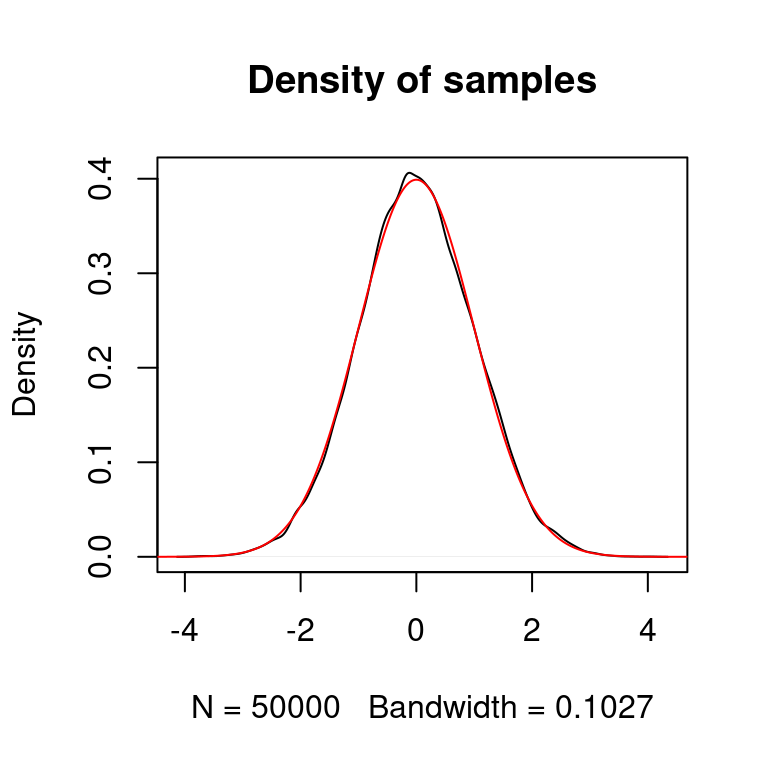
Our target distribution need not be one which is given by R. In practice the distributions we need to sample from are much more complex than the toy problems presented here. Below we sample from a mixture distribution: The weighted mixture of two normal distributions \(Z \sim 0.6X + 0.4Y\), where \(X \sim N(-2,1)\), \(Y \sim N(5, 2^2)\). We use a \(N(0,2^2)\) proposal distribution.
# generate markov chain using MH algorithm
# target: mixture of two normals
n <- 1e4
target <- function(x) {0.6*dnorm(x, -2, 1) + 0.4*dnorm(x, 5, 2)}
xs <- simulate.chain(make.metropolis.hastings.kernel(target,
                                                     make.normal.proposal(2)), 10, n)

# setup plot space
par(mfrow=c(1,2))

# plot the chain
plot(1:n, xs, type = 'l', xlab="iteration",
     main="Trace of Markov chain")

# plot the density of the chain
plot(density(xs), main = "Density of samples")
seq <- seq(-20,20,length.out=1e5)
lines(seq, target(seq), col="red")
The Metropolis-Hastings algorithm can also be used to draw samples from multi-variate distributions. Below we attempt to draw samples from a mixture of two 2D multivariate normal distributions. The contour plots highlight areas of the state space with high probability, and the path overlaid shows the steps that the MH algorithm has taken.
# higher-dimensional problem --- target: 2D multivariate normal distributions
# construct target
dmvnorm <- function(x, mu, sigma) return(as.vector(
  exp(-t(x - mu) %*% solve(sigma) %*% (x - mu)/2)/sqrt((2*pi)^length(x)*det(sigma))
  ))
mu1 <- c(2,2); mu2 <- c(-1,-1)
sigma1 <- matrix(c(1,0.3,0.3,1),2,2); sigma2 <- matrix(c(1,-0.1,-0.1,1),2,2)
target <- function(x) return(dmvnorm(x, mu1, sigma1) + dmvnorm(x, mu2, sigma2))

# evaluate density of target over grid
seq <- seq(-5,6,length.out=5e2)
mat <- outer(seq, seq, Vectorize(function(x, y) target(c(x,y))))
rownames(mat) <- colnames(mat) <- seq

# make contour plot
longmat <- melt(mat) #reshape data
## Warning in type.convert.default(X[[i]], ...): 'as.is' should be specified by the
## caller; using TRUE
## Warning in type.convert.default(X[[i]], ...): 'as.is' should be specified by the
## caller; using TRUEp1 <- longmat %>%
ggplot() +
geom_raster(aes(x = X1, y = X2, fill = value)) +
geom_contour(aes(x = X1, y = X2, z = value), col = "white") +
labs(title="Contour plot of the target")
# simulate chain
n <- 300
xs <- simulate.chain(make.metropolis.hastings.kernel(target,
make.normal.proposal(3)), c(-5,0), n)
# make plot of chain over contour
p2 <- longmat %>%
ggplot() +
geom_raster(aes(x = X1, y = X2, fill = value)) +
geom_contour(aes(x = X1, y = X2, z = value), col = "white") +
geom_path(data = as.data.frame(xs), aes(x=V1, y = V2), col="red") +
geom_point(data = as.data.frame(xs),
aes(x=V1, y = V2), pch=21, fill="red", col="white") +
labs(title="Contour plot of the target")
# plot p1, p2 side-by-side
grid.arrange(p1,p2,ncol=2)
MCMC in practice
Implementing MCMC methods in practice can be quite simple, but there are a few things that we need to be aware of to ensure that our algorithm is working well.
First we introduce the concept of pseudo-convergence. This occurs when there are regions of the state space with high probability that are poorly connected by the Markov chain. The chain may spend a long time exploring one high probability region, which falsely leads us to believe that the chain has converged to the stationary distribution. This phenomenon occurs frequently with multimodal distributions as we demonstrate below. If the modes are so far from one another such that the proposal distribution cannot propose values in one high-probability region when in another, the chain will fail to converge.
In the example below we attempt to sample from a univariate bimodal distribution. In the first scenario, we use a uniform proposal distribution with an interval length such that the chain cannot travel between modes. We repeat the simulation but with a larger interval for the proposal distribution.
# target: sum of two uniform densities
# proposal with interval length 2
n <- 1e3
target <- function(x) {0.5*dunif(x, -2,-1) + 0.5*dunif(x, 1, 2)}
xs <- simulate.chain(make.metropolis.hastings.kernel(target,
                                                     make.uniform.proposal(2)), 2, n)

# setup plot space
par(mfrow=c(1,2))

# plot the chain
plot(xs, type = 'l', ylim=c(-2,2), xlab="iteration",
     main="Trace of Markov chain")

# plot the density of the chain
plot(density(xs), main = "Density of samples", xlim=c(-3,3))
seq <- seq(-20,20,length.out=1e5)
lines(seq, target(seq), col="red")
# target: sum of two uniform densities
# proposal with interval length 5
n <- 1e4
target <- function(x) {0.5*dunif(x, -2,-1) + 0.5*dunif(x, 1, 2)}
xs <- simulate.chain(make.metropolis.hastings.kernel(target,
                                                     make.uniform.proposal(5)), 2, n)

# setup plot space
par(mfrow=c(1,2))

# plot the chain
plot(xs, type = 'l', ylim=c(-2,2), xlab="iteration",
     main="Trace of Markov chain")

# plot the density of the chain
plot(density(xs), main = "Density of samples", xlim=c(-3,3))
seq <- seq(-20,20,length.out=1e5)
lines(seq, target(seq), col="red")
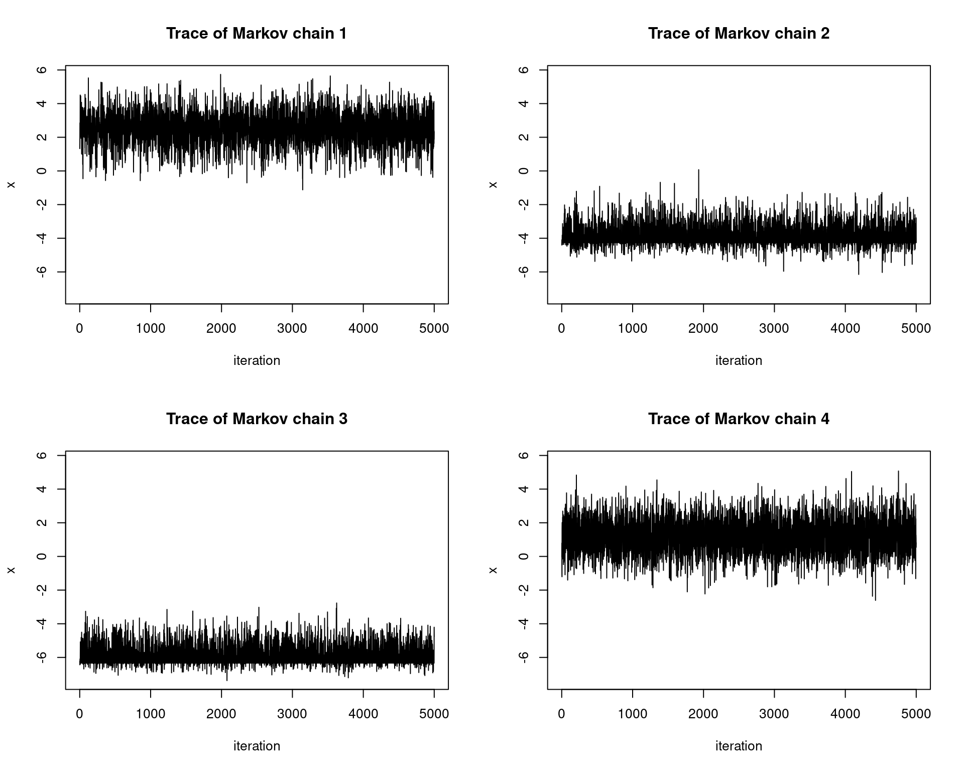
One way that we may attempt to overcome the pseudo-convergence phenomenon is to run multiple chains. This simply means that we run the MCMC algorithm multiple times with different initializations. If the chain seems to have converged to different distributions for different initializations, then the algorithm has failed to fully explore the state space. We may need to run the chain for a longer period of time until it converges to the target distribution, or we may need to adjust the proposal distribution to improve the chain’s mixing. This introduces a new problem: given a fixed amount of computation, should we produce one long chain or multiple chains? This `multistart heuristic’ should be used with caution — it only guarantees against pseudo-convergence if we can ensure that the starting points cover every part of the state space which may pseudo-converge.
Another practical aspect of MCMC methods that we should be aware of is burn-in. When initializing our algorithm it may take some time before the Markov chain converges to a stationary distribution, and we call this the burn-in period. The samples produced before the chain has converged are not likely to have been produced by the target distribution, and so we discard these samples. The best way to see which samples to discard is to manually inspect the chain in order to see at which iteration it began to converge.
Below we parallelize our computations and run one chain per one physical CPU core. The details of the target distribution in this example do not matter — often we do not know them in practice — the point is that we can observe pseudo-convergence in the trace plots of the chains. This occurs because our proposal distribution has a small variance and thus the chains cannot fully explore the state space.
simulate.chains <- function(P, x0, n, n.chains, n.cores = 4) {
  require(parallel)
  require(doParallel)
  # parallelize chains
  registerDoParallel(n.cores)
  simulations <- foreach(i=1:n.chains, .combine="rbind") %dopar% {
    x <- x0[i]
    foreach(i=1:n, .combine="c") %do% {P(x)}
  }
  stopImplicitCluster()
  return(simulations)
}

# generate markov chain using MH algorithm
# target: mixture of two normals
n <- 5e3; set.seed(123)
target <- function(x) {0.6*dnorm(x, -2, 1) + 0.4*dnorm(x, 5, 2)}
xs <- simulate.chains(make.metropolis.hastings.kernel(target,
                                                      make.normal.proposal(1)),
                      runif(4,-10,10), n, 4)
## Loading required package: parallel## Loading required package: doParallel## Loading required package: foreach##
## Attaching package: 'foreach'## The following objects are masked from 'package:purrr':
##
## accumulate, when## Loading required package: iterators# setup plot space
par(mfrow=c(2,2))
# plot the chains
ylimits <- c(min(xs), max(xs))
for(i in 1:4){
plot(1:n, xs[i,], type = 'l', xlab="iteration", ylim=ylimits,
ylab="x", main=paste0("Trace of Markov chain ", i))
}